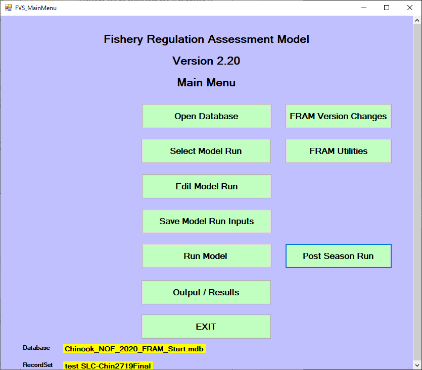
Main menu screen
After launching FRAM and
continuing past the startup splash screen, the main menu organizes the
available functionality. Below are links to sections that correspond to
different main menu items as well as descriptions of some of the primary
files associated with preparing and conducting runs.

- Open Database is the first step to using FRAM, opening a
file selection window to choose a [Project database]
- FRAM Version
Changes opens a window with summary text descriptions of the
present and past versions
- Select Model Run allows the choice of a particular
model run and associated parameters from the [Project database];
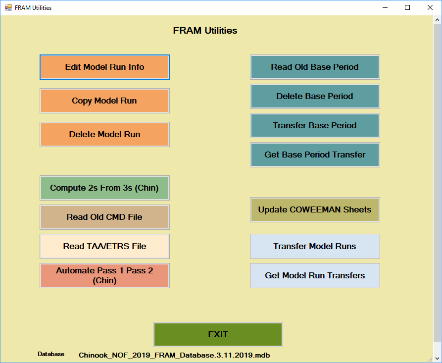
- FRAM Utilities opens a secondary menu of tools
for managing files and runs
- Edit Model Run opens
a secondary menu with options to alter stock and fishery parameters for
the currently selected run
- Save Model Run
Inputs ensures that changes to values in memory are written
to the appropriate [Project database tables]
- Run Model triggers the
calculation of outputs given the current parameter values and
conditioned on several final choices
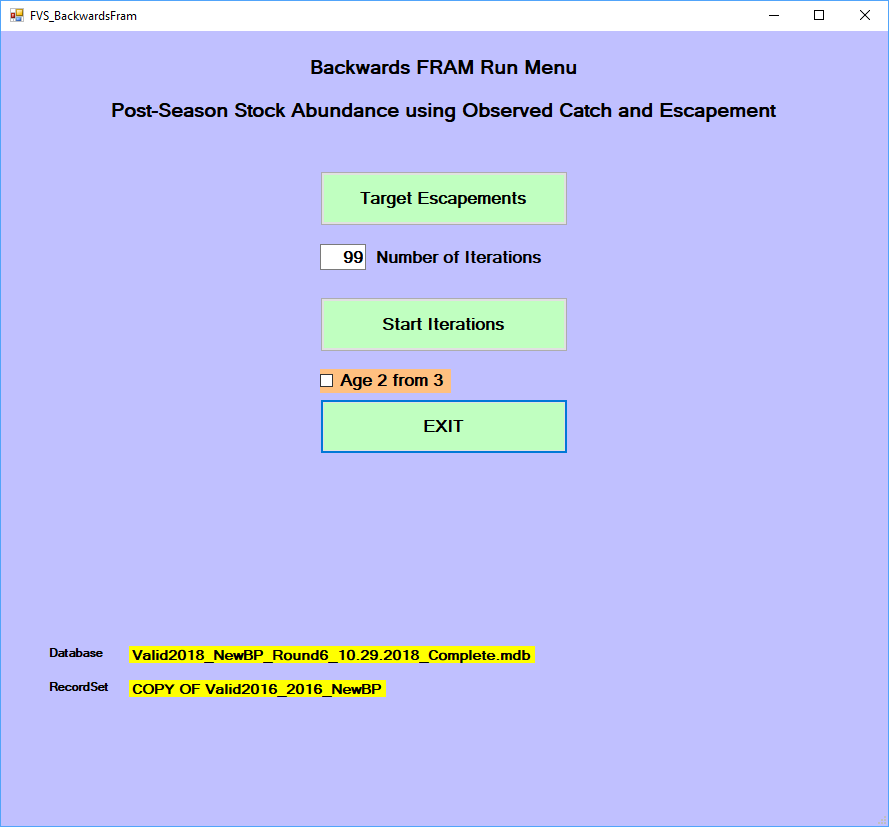
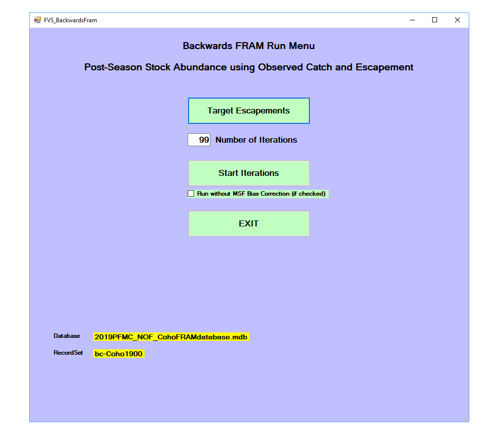
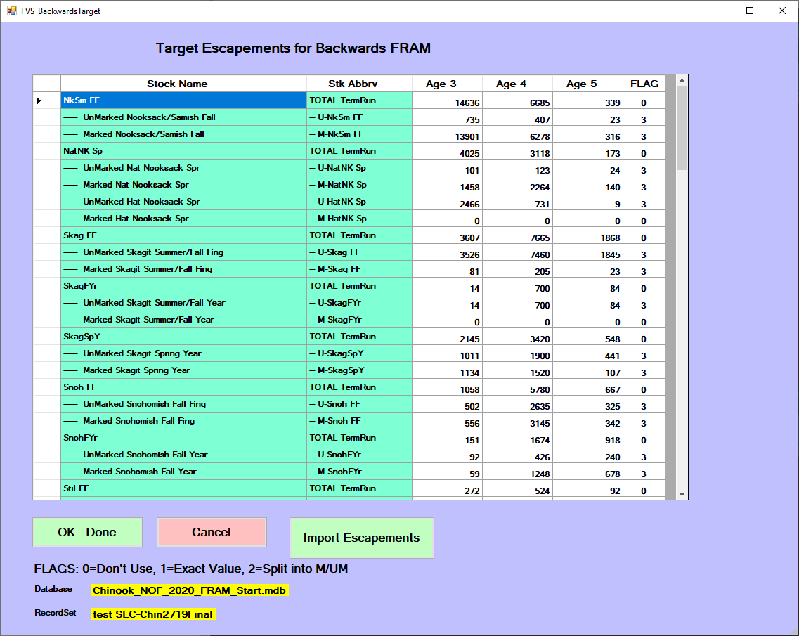
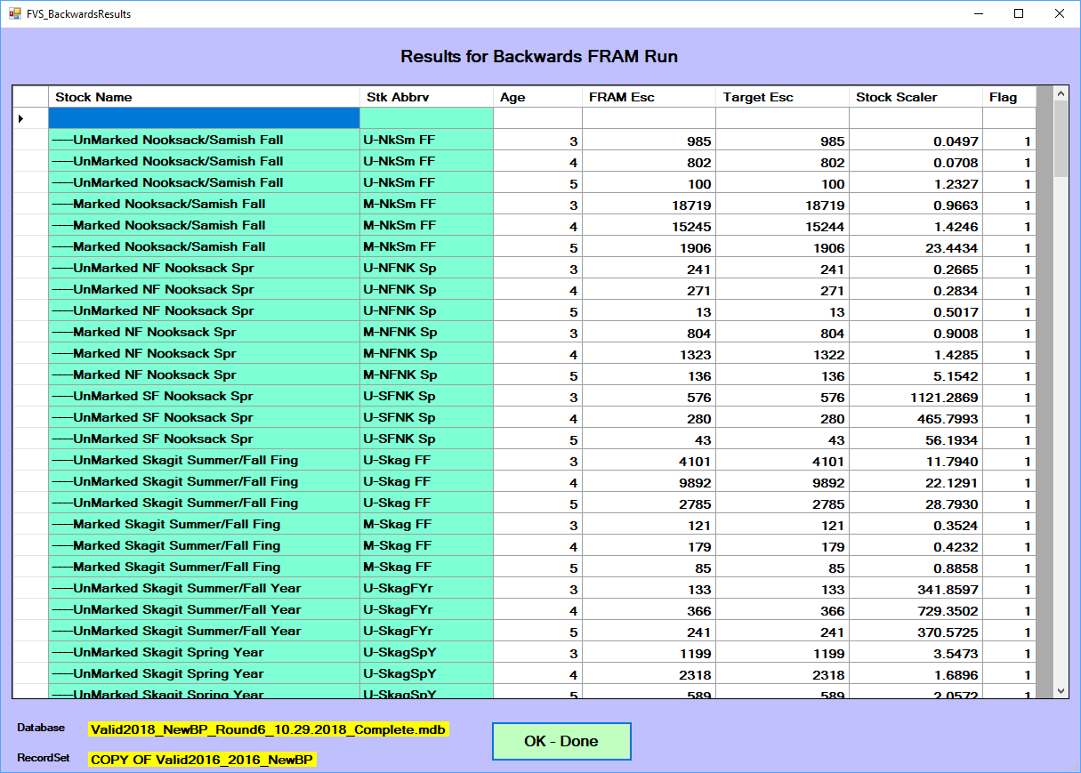
- Post Season Run initiates the process of a Backwards FRAM run
(not necessarily during the post-season) that uses catch and terminal
abundance to reconstruct pre-fishing cohorts
- Output/Results opens a secondary menu allowing
selection of various [Outputs] following model run completion
- Exit closes the program
Edit model run
FRAM
allows users to explore different management scenarios by adjusting
“inputs” ([Per-run parameters]) that control fishery and stock
properties.
For some analyses, it may make sense to adjust model parameters
outside of the FRAM
application. For example, a uniform increase or decrease in a group of
fisheries over multiple time steps may be accomplished more easily by
manipulating the project database directly.
However, the main menu “Edit model run” button accesses a convenient
interface for changing individual values within the application.
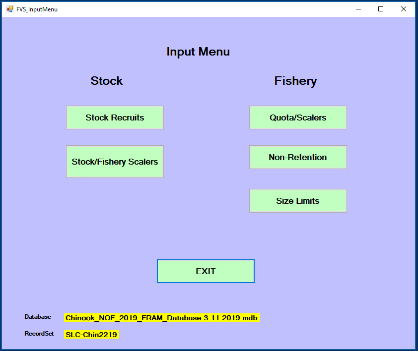
Clicking this produces a submenu divided into further “Stock” and
“Fishery” buttons.

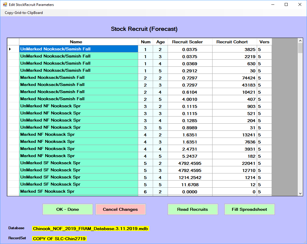
Stock recruits
Stock recruit scalers (StockRecruit in [Per-run
parameters]) are multiplied against a base period abundance
(BaseCohort in [Base period parameters]) to generate a
starting, pre-fishing cohort by stock (and age for Chinook).
These parameters represent the magnitude of the current stock
abundance relative to that during the base period years. Thus, a stock
recruit scaler of 1 indicates an annual abundance for that stock equal
to the base period, a value >1 is an abundance larger than the base
period, and <1 is an abundance smaller than the base period.
Coho ‘Recruit Cohort’ values are in January age-3 units, whereas
Chinook ‘Recruit Cohort’ contains four age-class specific initial ocean
abundance values.
For preseason forward runs, stock recruit scaler values are a
function of stock-specific forecasts provided by technical staff at the
beginning of the planning cycle. They are generally established at the
outset of preseason planning and then updated if necessary as additional
data are available for the year (i.e. Canadian Chinook forecasts are not
usually available until the end of March). For Chinook, stock recruit
scalers are typically produced from terminal run size forecasts by
running Backwards FRAM.
Accordingly, recruit scalers would not usually be manually adjusted
during a typical forward model run, but the interface enables this
possibility if, for example, one wanted to explore the implications of a
much larger or smaller salmon return than was predicted or with a
different age distribution (e.g., “what happens if stock X returns at
half of what was forecast and/or with far more younger fish?”).
Note that updating the stock recruit scaler will automatically update
the associated recruit cohort and vice versa.
The “Read Recruits” button can be used to load forecast values
compiled in the external FRAMVSTemplate file from sheet FRAM_Recruits.
Conversely, the “Fill Spreadsheet” button can be used to download values
from the model run to the FRAMVSTemplate file, where additional notation
or comments can be stored.

Stock/Fishery Scalers
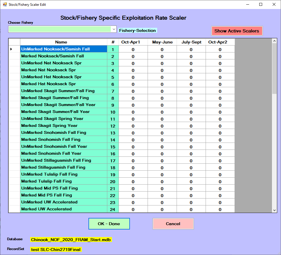
Stock-fishery-specific exploitation rate (ER) scalers allow adjustments to
the base period directed impacts of a particular fishery on a specific
stock or group of stocks within each time step. These scalers function
act on the base period fishery-stock-specific ERs.
These parameters can provide a temporary fix to an identified issue
in the FRAM base
period calibration. They are also used to represent negotiated closures
within a fishery (e.g. a spatial closure). Any such adjustments must be
supported by an accepted external analysis of fishery-stock interactions
which demonstrates how and why the fishery would be expected to have
different stock-specific contribution levels than it had during the base
period years (e.g. CWT
recoveries or genetic stock identification).
Stock-fishery-specific ER
scalers display 0 until a fishery is selected from the upper left
drop-down menu.
If a fishery/time-step is not modeled, a “****” is displayed with
blue highlight.
By default, the values are equal to 1, which means the base period
exploitation rate is used. Thus, a value >1 is a larger ER than the base period and <1 is
smaller than the base period ER.
After choosing the focal fishery, the desired values are directly
input into each cell and the “Ok - Done” button writes those changes to
the project database for the active model run. These changes then
persist across subsequently copied runs.
Few to none of these scalers may be “actively” modifying the many
possible stock-fishery combinations in a FRAM run, and
the red “Show Active Scalers” button presents a secondary screen
filtered to and highlighting those particular instances. Although values
cannot be directly modified on this screen, it can serve as a useful
check of the current model run parameterization.
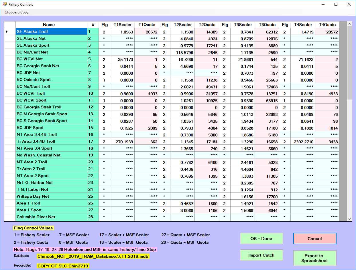
Fishery Quota/Scalers
These [Per-run parameters] control the representation of fishery
effort and may be the most frequently adjusted FRAM element
during preseason planning.
As noted in the [Edit input parameter values] section of [A Basic
Forward Run], legal, landed catch fishery impacts are controlled by
“quotas” and/or “scalers” which are in turn controlled by per-timestep
fishery flags. Values entered or adjusted under the
quota/scalers input menus are stored in the [Project database tables]
FisheryScalers. Fisheries without an input will be modeled
with a default fishery effort scaler of 0.0 (flag = 1).
The flag values (displayed in the interface) determine whether the
fishery is treated as non-selective and/or mark selective, and whether
catch is processed as a fixed expectation (quotas) or as effort relative
to the base period (scalers). Both modes operate on the fishery as a
whole, combining with stock and age specific exploitation rates to
determine resulting impacts from the fishery.
Note that many fishery/time-step cells are filled with asterisks
(****) designating a lack of base period information to model that
stratum. If a fishery now operates in one of those time steps the input
(and impacts) need to be combined with an adjacent fishery or time
step.
A single value in the input interface (either a scaler or quota) can
be entered, and once the model is run, the resulting associated value
will be populated in the interface (e.g. enter a quota value here and
proceed through the menus to complete a model run, which will then
return the resulting scaler value for that entered quota). Several
values can be entered or updated before clicking “OK – Done”.
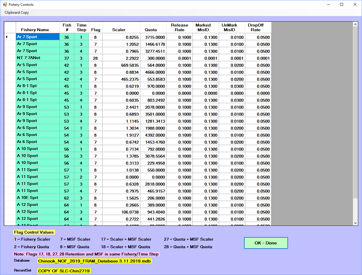
The values for mark-selective fisheries are displayed on a secondary
input screen that is displayed after selecting “Ok - done”. Only fishery
and time steps flagged in the first fishery controls screen as
mark-selective or a combination with a mark-selective component will be
present in the secondary MSF input screen (flags 7, 8,
17, 18, 27,28; displaying a magenta highlight in Scaler/Quota cells).
Thus, if you want to enter a MSF or change a MSF input parameter, be sure
it is flagged as such first.
In addition to scaler and quota inputs, the MSF fishery controls input
screen also contains four additional input parameters. Some of these
parameters are derived and agreed-to each preseason planning cycle by
salmon co-managers and others are set by the PFMC management
process. Thus, some stay fairly static year-to-year and some change
annually.
- Release Rate: Hooking release mortality rate (landed fish then
released)
- Marked MisID: Release rate of marked fish that could be legally
retained
- UnMark MisID: Retention rate of unmarked fish that should have been
released
- DropOff Rate: Fishery-related mortality rate (fish that escape but
die due to injury)
Note these four MSF
input parameters cannot have a zero value and must be >0.0000.
Altering a fishery quota has fairly intuitive
implications (though the target value may itself result from
considerable additional calculation external to FRAM). In
contrast, the particular numeric effects of altering
fishery scalers requires more prior knowledge of the base
period practices (and stock composition).
In addition to the direct adjustment of single values in the
interface (which are then written to the database), the “Import catch”
and “Export to spreadsheet” buttons provide functionality to read and
write values for all fisheries and time steps at once from an external
[FRAMVSTemplate file], on sheets FRAMinput and FRAM_MSF. Note also the
“clipboard copy” option in the upper left corner of the interface.
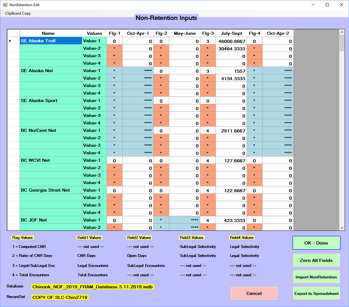
Non-Retention
Coho or Chinook non-retention (CNR) inputs represent any
fishery (or portion of a fishery) that will be open for salmon fishing
but requires release of Coho or Chinook. Differences in the input menu
screens for Coho and Chinook reflect the different methodologies.
For Chinook, similar to other inputs, control flag values (flags 1 –
4) determine the mode by which non-retention impacts are calculated,
with different modes requiring various additional parameter values
(Field1, Field2, Field3, Field4) (definitions displayed in the lower
left of the interface window). Typically, only flag 3 (Legal/Sublegal
Encounters) or flag 4 (Total Encounters) are used. Encounters for Puget
Sound marine sport fisheries can be automatically updated using the
[Automate Pass 1 Pass 2] button on the FRAM Utilities menu.
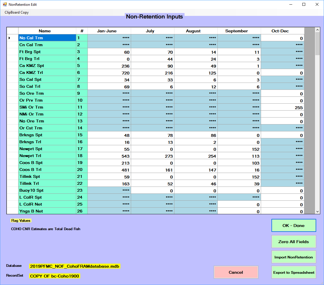
For Coho, non-retention mortality is calculated outside of the model
and entered as the total number of dead fish resulting from the
non-retention portion of a fishery/time-step. Typically, the value is
derived from a historic level of landed or encountered coho and then
applying both a release mortality rate and a drop-off mortality rate to
that historic level, and summing the two types of mortalities.
Similarly, the individual values can be altered (and consequently
saved to the run in the database) and there is also a button to “Zero
All Fields”. In addition, the interface provides options to “Import
NonRetention” and “Export to Spreadsheet” all fishery/time steps from
the external FRAMVSTemplate file (sheet FRAM_CNR).
Note many fishery/time-step cells are filled with asterisks (****)
designating a lack of base period information to model that stratum. If
a fishery now operates in one of those time steps the input (and
impacts) need to be combined with an adjacent fishery or time step.
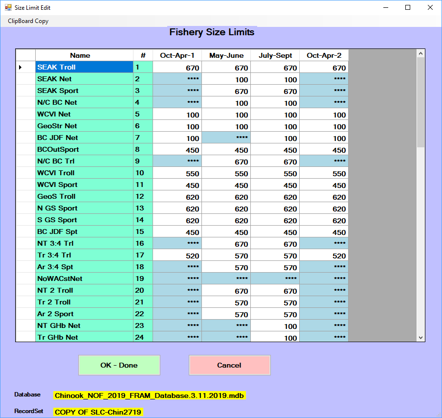
Size Limits (Chinook)
The minimum length of legal landed catch is defined per-fishery and
time-step. This is relevant for multi-aged Chinook modeling where the
minimum retention size limit (unit = fork length in millimeters) may
vary annually, by fishery and/or by time-step. Generally:
- troll fisheries often require larger fish than sport in the same
location and time
- winter limits are often smaller
Run Model
This menu item initiates a model run - applying the current
parameters and input values to produce new output values.
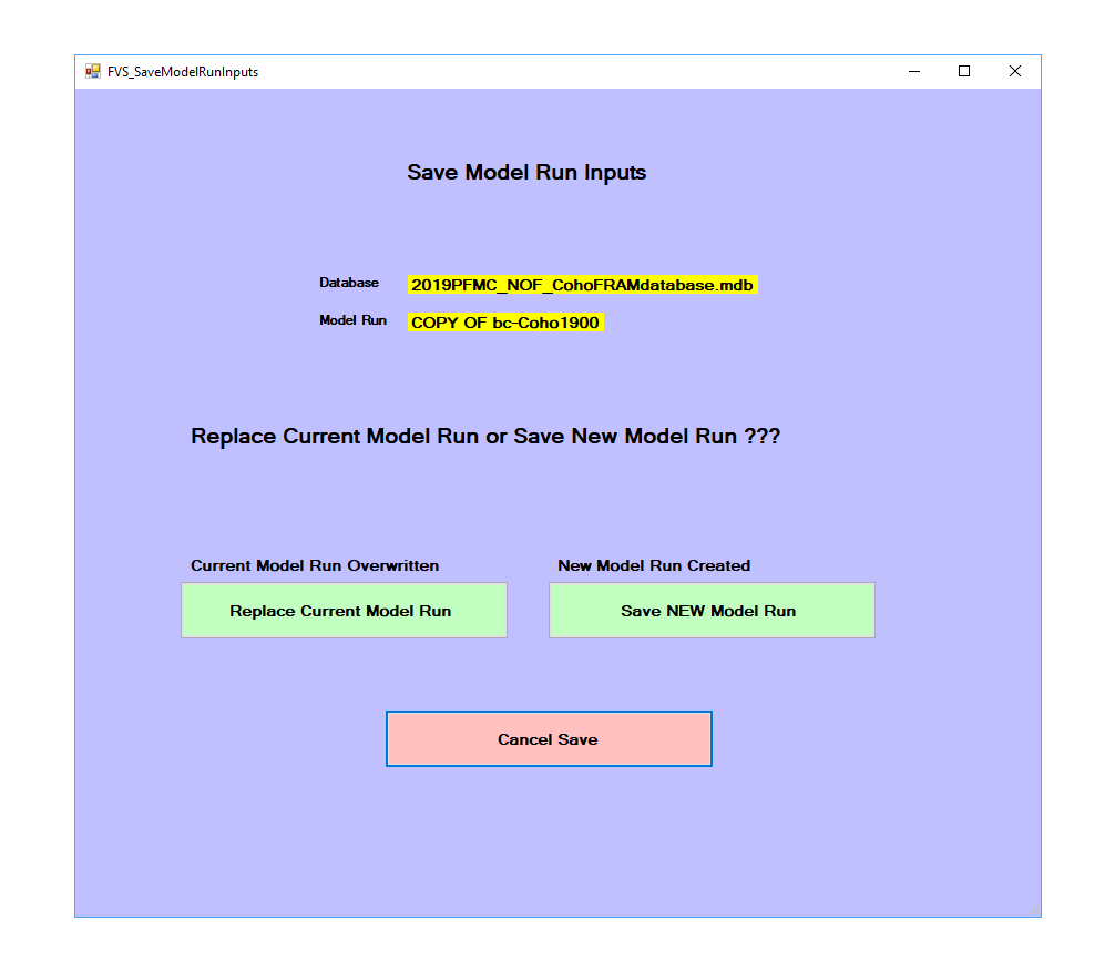
The application monitors when a user may have altered values relative
to the currently loaded run. If “Run Model” is selected when input
values have changed but have not yet been saved to the project database
tables associated with the model run, then a pop-up window will prompt
with the message “Input Values Have Been Changed! Changes Must be Saved
before Running Model!!! Save Current Model Run???”.
If you select “Yes” and save your model inputs by replacing the
current model run or creating a new model run, then when you click “Run
Model” from the Main Menu, it will present the Model Run Specifications
menu.
If you select the “No”, a message will warn you “Please be aware that
the OUTPUT for this model run cannot be duplicated without saving your
INPUT values.” If you click “OK”, then it will present the Model Run
Specifications menu.
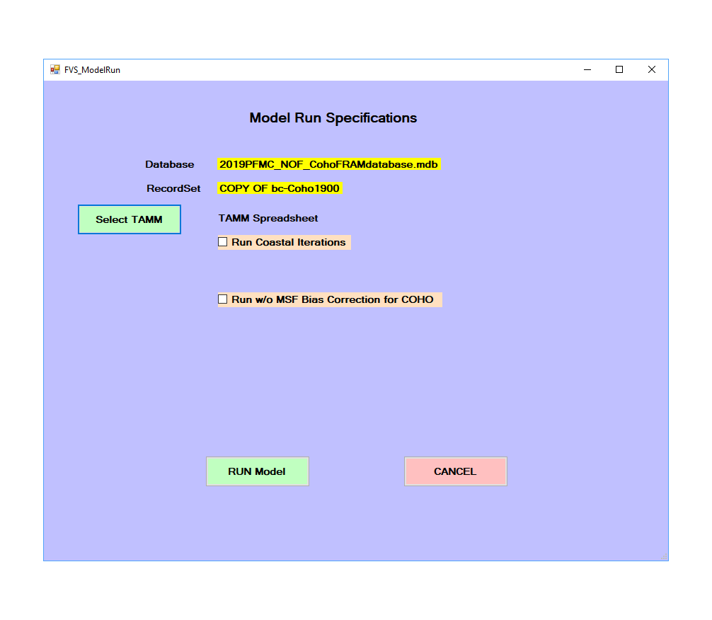
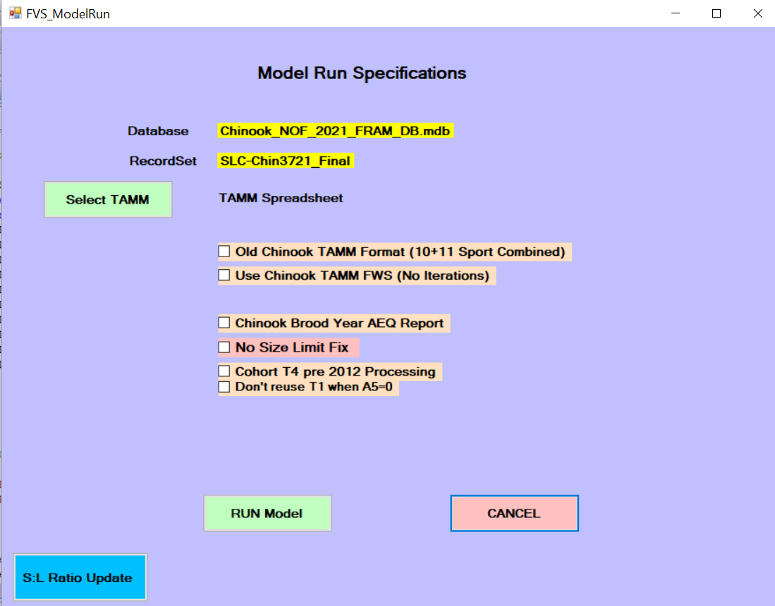
The forwards FRAM Model Run
Specifications menu screens include several optional checkboxes which
differ by species. The sections below describe these in more detail.
The “Select TAMM” button is
used to navigate to and select an associated TAMM file (see
also Running FRAM with TAMM). Note
that when a model run with a TAMM begins, the
prompt “Do you want to save TAMM Transfer
Values into TAMM spreadsheet?”
will apear. Choosing “Yes” will ensure TAMX values
are updated. After run completion, the TAMM file used will
include updated values and be open, though possibly in the background.
Make sure to navigate to the open TAMM file and save
it to retain the modeled values.
Once the model run is complete, the model run name may have been
updated with a prefix in the list of model runs within a database (Main
Menu – Select Model Run to see list). For coho, the prefix “bc-“ is
added when the default calculations for MSF bias correction have been
used in a model run. For Chinook, the prefix “SLC-“ is added when the
default calculations for size limit fix have been used in a model
run.
Coho
Run coastal iterations
Beginning with the 2017 preseason, FRAM was
updated to automate a previously manual process of iterating Washington
coastal terminal fishery inputs between TAMM and FRAM. The
fishery inputs are read into FRAM from a
formatted table on TAMM sheet
WACoastTerminal (starting row 150, cells in green highlight, as landed
catch; flag 2 = fishery quota) and iterated to ± 1 fish.
When working with a Coho project database, from the main menu “Run
Model” button, the Model Run Specifications screen requires you to
select the TAMM file
associated with the model run and then select the checkbox for “Run
Coastal Iterations” before clicking the “RUN Model” button to complete
the process.
By default, this checkbox should be used/checked with all preseason
Coho model runs, as Washington coastal iterations are needed every time
a terminal area’s fishery structure changes or when a pre-terminal FRAM fishery
changes the ocean escapement value.
In general, FRAM produces
an ocean escapement for each Washington coastal coho stock and regional
technical staff utilize those values in regional terminal harvest
management models. The local stock-specific harvest rates from the
regional terminal models are then utilized in the WACoastTerminal sheet
of the TAMM
and in subsequent calculations. These results differ from the base
period exploitation rates used in FRAM.
However, FRAM is used
with base period stock composition for associated impacts upon non-local
stocks in terminal regional fisheries with “dip-ins” (i.e. fish which
could be expected to return to their native systems if not harvested;
not a stray).
Thus, the final results of stock impacts in Washington coastal
terminal fisheries are a combination of regional specific local stock
impacts and those produced by the FRAM and its
base period.
Run without MSF
bias correction
By default, a mark-selective fishery bias correction factor is used
in both preseason and post-season Coho FRAM modeling.
The MSF bias correction
in FRAM
was a result of demonstrating that unmarked mortalities were
underestimated due to multiple encounter bias from mark-selective
fisheries [@conrad2010] and the desire to
incorporate bias-corrected equations into FRAM [@conrad2011, @ahb2012].
The checkbox “Run w/o MSF Bias Correction” should
not be checked except in unusual circumstances or for troubleshooting
purposes. As a result of the MSF bias correction factor
calculations in FRAM, the
program will often prompt the user with a warning that a particular
stock has exceeded 100% ER
(i.e. the stock size has gone negative in the model and at what point).
This is often helpful in troubleshooting issues with fishery inputs.
Chinook
Use Chinook TAMM FWS (No
Iterations)
Selecting this button when running FRAM with TAMM will not load
TAMI values into FRAM, yet load
TAMX output into TAMM. Existing
FRAM
terminal fishery values will be used to run FRAM. TAMM iterations
will not be performed.
This button is rarely used, but can be a helpful shortcut when
needing TAMM
output, but TAMM terminal
fishery inputs are not available. Compiling information for a long time
series of post-season runs is an example of where this procedure may be
beneficial. TAMM consolidates a
multitude of terminal fishery inputs into just a few key TAMI values.
These fewer, consolidated values are easier to compile than the detailed
TAMM inputs
(e.g., avoiding splitting post-season catches into regulation periods
for sockeye, coho, chum etc.). Terminal fishery catches can be directly
entered into FRAM. As long
as TAMM
contains updated terminal run sizes and freshwater inputs, TAMX output
will be compatible with the TAMM it is loaded
into.
Chinook Brood Year AEQ
Report
Selecting this check box produces a brood year exploitation rate
report called “BY-Cohort-Compare-FramVS.txt” located in the same
directory as the FRAM
database.
Brood year calculations subject the forecast abundance of an age to
the current fishing year’s fishery inputs, calculate the resulting
escapement as well as the number of fish remaining in the ocean and
advance to the next age. The resulting age+1 is then also subjected to
the same fishery inputs, until age 5 is reached. Thus the same fishery
inputs are used for all four ages (2-5) resulting from a brood year.
FRAM
algorithms are applied to each age class in forward and reverse
mode.
Note that, in contrast, a “true” brood year run would apply fishery
inputs from the first year to age 2s, compute the resulting age 3s,
apply fishery inputs from year+1 to these age 3s, compute the resulting
age 4s, apply fishery inputs from year+2 to these age 4s, compute the
resulting age 5s, and finally apply fishery inputs from year+3 to the
age 5s.
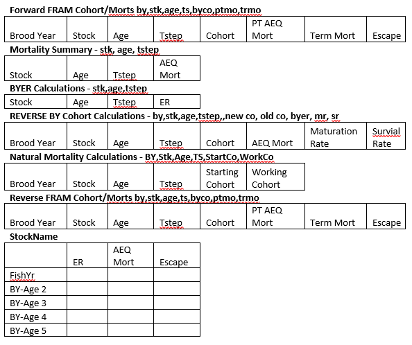
Forward and reverse brood year computations by age; i.e. calculate
age 2 starting cohort for age 3 forecast with reverse calculations, then
calculate age 4 and 5 starting cohort with forward calculations.
This then generates a report with this type of information:
No size limit fix
FRAM
allows for evaluations of the effect of changes in minimum size limit
regulations to fishery catches and stock impacts. Size limits are
altered infrequently in hook and line salmon fisheries. FRAM’s original
size limit evaluation algorithms were problematic, because they resulted
in changes to the number of total encounters with each size limit
change. FRAM uses
different rates to model encounters of legal and sublegal fish. These
rates are computed during the calibration process and are based on
landed catch and encounter information during base period years
(currently brood years 2005-2008).
When size limits are modeled in FRAM, each fish
smaller than the size limit is treated as a sublegal fish. Sublegal
encounter rates are used to compute releases and release mortalities.
Conversely, each fish larger than the size limit is deemed legal and
legal encounter rates are used to estimate catch as well as releases and
release mortalities in mark selective fisheries. As the size limit is
changed, a portion of the population (with sizes between the old and the
new size limit) that previously received a sublegal encounter rate will
receive a legal encounter rate or vice versa. Because legal and sublegal
encounter rates are not the same for the same stock and age, this leads
to the total number of computed encounters varying with size limits, an
incorrect outcome, if effort remains constant.
FRAM
incorporates corrected equations that hold total encounters constant,
regardless of the modeled size limit (@ahb2013, @mchugh2015, @johnson2015).
In a first round of evaluations, FRAM computes
sublegal encounters using sublegal/legal ratios based on recent field
data (i.e., length-frequency data for Chinook encounters in recreational
test fisheries). These ratios are updated each year in the [Project
database tables] “SLRatio”. To produce the desired sublegal encounters,
FRAM
iteratively calculates an “Encounter Rate Adjustment” for each fishery
and time step, such that sublegal encounters summed over stocks and ages
within a fishery and time step produce the target sublegal/legal ratios,
given legal sized, landed catch inputs (fishery scalers or quotas). Once
run, “Encounter Rate Adjustments” are stored in the
“RunEncounterRateAdjustment” column of the “SLRatio” table.
Size limit changes are evaluated with Van Bertalanffy growth
equations. These equations determine the proportion legal and
or/sublegal by stock and age under desired size limit regulations. The
model calculates the legal and sublegal encounters for both the original
and new minimum size limit and then adjust the differences so that total
encounters remain constant.
When the new size limit is less than the base-period size limit, the
difference in sublegal encounters between the base size-limit and the
new size-limit becomes landed catch that is added to the calculated
landed catch evaluated at the base-period size limit. Encounters are
calculated by dividing the encounter estimates by the sublegal release
mortality rate.
Conversely, when the new size limit is greater than the base-period
size limit, the difference in landed catch between the new size limit
and the base-period size limit becomes sublegal encounters. This
encounter difference is added to the calculated sublegal encounters from
the base-period size limit to get total sublegal encounter
mortality.
When this button is checked, FRAM will not
automatically update the encounter rate adjustments needed to achieve
desired sublegal/legal ratios and instead use the encounter rate
adjustments in the existing model run. FRAM will also
revert to original size limit evaluation algorithms, where total
encounters can fluctuate when size limits are changed.
If unsure, please leave this button unchecked (default), as the
default setting will produce the most accurate run. However, there are
several reasons to check the “No-Size-Limit-Fix” button:
- To speed up the run, as sublegal encounter iterations, especially
when performed with TAMM, can be very
time consuming. However, for correct results, the following assumptions
need to be met:
- “Encounter Rate Adjustments” were updated during a previous model
run and will result in desired sublegal/legal ratios (see Background
paragraph above).
- The sublegal/legal ratios in the database were computed for the same
size limits that exist in the current model run.
- For backwards compatibility to reproduce an “old-style” (pre 2013)
run
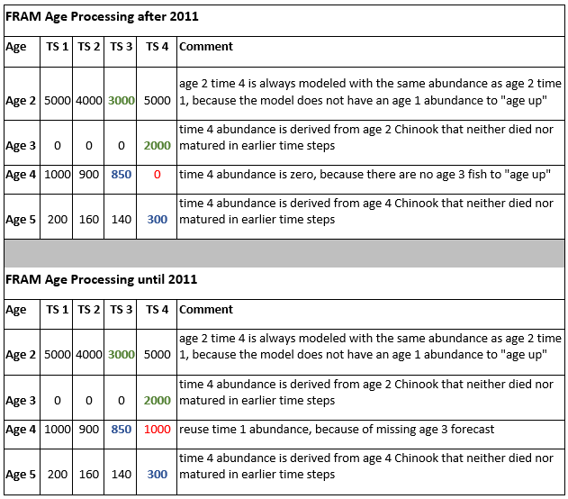
Cohort T4 pre 2012 Processing
This button exists for backwards compatibility reasons. Prior to
2012, FRAM would not
have reused time step 1 forecasts in time step 4 for ages with a missing
“age minus 1” abundance. Chinook age up in time step 4; i.e. an age 2
fish becomes an age 3 fish, an age 3 fish turns age 4, etc. Previously,
if a stock was not expected to return at a certain age, time 4 of age+1
would have been left blank. Since 2012, for these stocks, time step 4 of
a given age reuses the time step 1 abundance of the same age.
Don’t reuse T1 when A5 = 0
The “Don’t reuse T1 when A5=0” button was added for backwards
compatibility of runs constructed between 2012 and 2021. When the
corrections in the previous paragraph were implemented, the modelers
added a provision to prevent re-use of time 1 abundances in time 4, when
age 5 abundance was zero. The extra condition was added to prevent
recycling ages that are actually the end of days for a particular stock
or single brood production case. It is however much more common for
stocks to miss an age 5 abundance than to be discontinued. Therefore,
this provision was eliminated. Checking the button re-instates the age 5
condition in order to reproduce runs conducted between 2012 and
2021.
S:L ratio update
Since 2014, FRAM computes
sublegal encounters using sublegal/legal ratios (@mchugh2015, @johnson2015). These ratios are usually derived
from recent field data (i.e., length-frequency data for Chinook
encounters in recreational test fisheries) and updated annually in the
“SLRatio” table of FRAM’s ACCESS
database. To produce the desired sublegal encounters, FRAM
iteratively calculates an “Encounter Rate Adjustment” for each fishery
and time step such that sublegal encounters summed over stocks and ages
within a fishery and time step produce the target sublegal/legal ratios,
given legal sized landed catch inputs (fishery scalers or quotas). Once
run, “Encounter Rate Adjustments” are stored in the
“RunEncounterRateAdjustment” column of the “SLRatio” table.
The “S:L Ratio Update” button is a relic from pre-2019 FRAM.exe
releases. The new FRAM default
(leave “No Size Limit Fix” button unchecked) automatically updates
Encounter Rate Adjustments with each model run in the course of
computing size limit corrected legal and sublegal encounters.
When this button is clicked, FRAM will
calculate “Encounter Rate Adjustments” for each fishery and time step
such that sublegal encounters summed over stocks and ages within a
fishery and time step produce the target sublegal/legal ratios. These
ratios are then stores in the “RunEncounterRateAdjustment” column of the
“SLRatio” table.
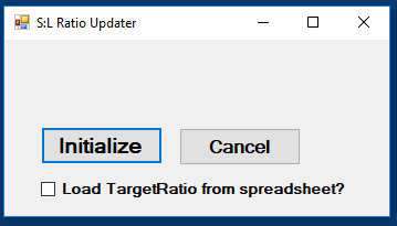
A message box will appear when clicking the “S:L Ratio Update”
button.

The user then has the option to check “Load TargetRatio from
spreadsheet” box before clicking the “Initialize” button. This brings up
a file selection dialog box. Choose the file with the desired
sublegal/legal ratios. The file will most likely have “SL Ratios…” in
the title and contain a tab called “SLRatioImport”. If the ratios are
already loaded, leave this box unchecked. As soon as the ratios are
loaded in the database, within a few seconds of clicking “Initialize”,
FRAM’s
“Run-Menu” will appear. Select the “Run Model” button to run FRAM as
usual.
Since “Encounter Rate Adjustments” are automatically updated in the
default mode, selecting this option only makes sense in combination with
clicking the “No Size Limit Fix” button. This results in a model run
with updated “Encounter Rate Adjustments”, but old size limit
evaluations. Doing so is only advisable if the user is sure that size
limits in the current model run are compatible with the sublegal/legal
ratios in the database. One other reason to select the “S:L Ratio
Update” button is the option to programmatically load target
sublegal/legal ratios from an Excel workbook as described above.
Output/Results
A FRAM
model run produces [Output values] that are stored in several [Project
database tables].
These results can be accessed and analyzed with external applications
such as R or Microsoft Excel, and this is often preferable when
addressing multiple model runs. For example, when examining a particular
stock or fishery across multiple model runs within a single project
database, the key tables can be joined and filtered to reach a focal
subset for further manipulation and visualization.
However, the FRAM
application also provides functionality to interactively view results
for a single run by selecting the main menu button
Output/Results.
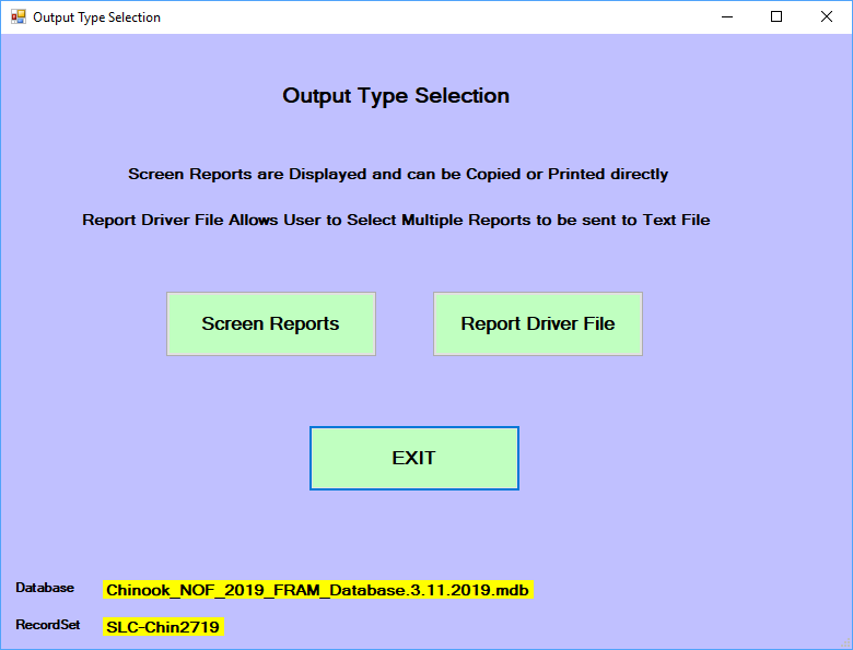
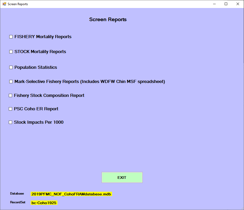
Screen reports
The “Output Type Selection” submenu offers
Screen Reports. Note that if all values are zero within
these reports, then the model must be run in the project database to
generate actual results.

Selecting this then displays several further options.

Select a screen report by clicking in the appropriate checkbox. Once
in view, note that many of these reports include a “clipboard copy”
option in the upper left corner. This allows the user to paste the data
into other external programs (e.g., Microsoft Word or Excel).
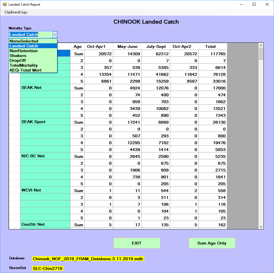
Fishery mortality reports
This view aggregates across stocks within a fishery, summarizing
different types of mortality. For Chinook, these values can be displayed
summed or broken out by age per fishery (i.e., all age 3 catch within
fishery N). Results may also be displayed as a zero value for strata in
which base period data are unavailable. In other screen reports, these
strata are often denoted with “****”.
Landed Catch designates fish that are caught and
retainedNonRetention includes incidental mortalities from
mark-selective fisheries and/or other fisheries not targeting Chinook or
coho (e.g., pink or chum salmon, test fishing, etc.)Shakers accounts for non-landed mortalities from
sub-legal encountersDropoff (also net drop out) represents mortality from
encounters in which the fish is never observed (i.e., “the one that got
away”)TotalMortality is the sum of these components- For Chinook,
AEQ-Total Mort designates the “adult
equivalent” translation of the total mortality, reflecting an age-based
estimate of the fish that could have actually survived to return to
spawn given subsequent years of fishing and non-fishing related impacts
(e.g., younger fish that are killed due to fishing in year Y would not
necessarily have survived to return in a later year Y+t, even in the
absence of year Y’s fishing)

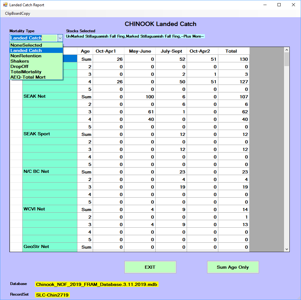
Stock mortality reports
The mortality types described above can also be viewed by fishery and
time step for an individual stock or a selected sub-set of stocks. After
selecting this report, a menu allows selection of a single stock or
multiple stocks using Control+Click. After the desired stocks are
highlighted, click “OK – Done” to view the report. The fishery mortality
data types will be summarized for all stocks selected.

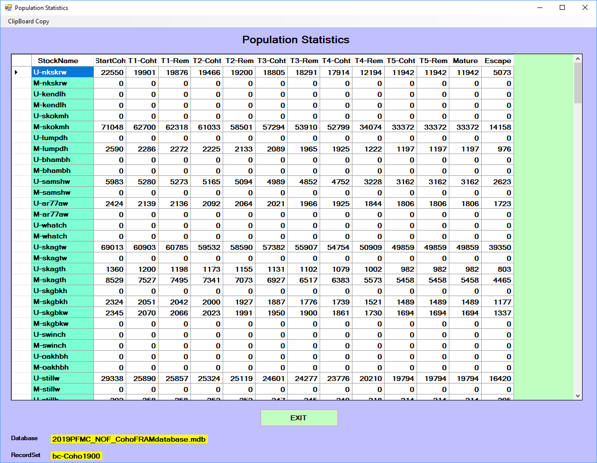
Population statistics
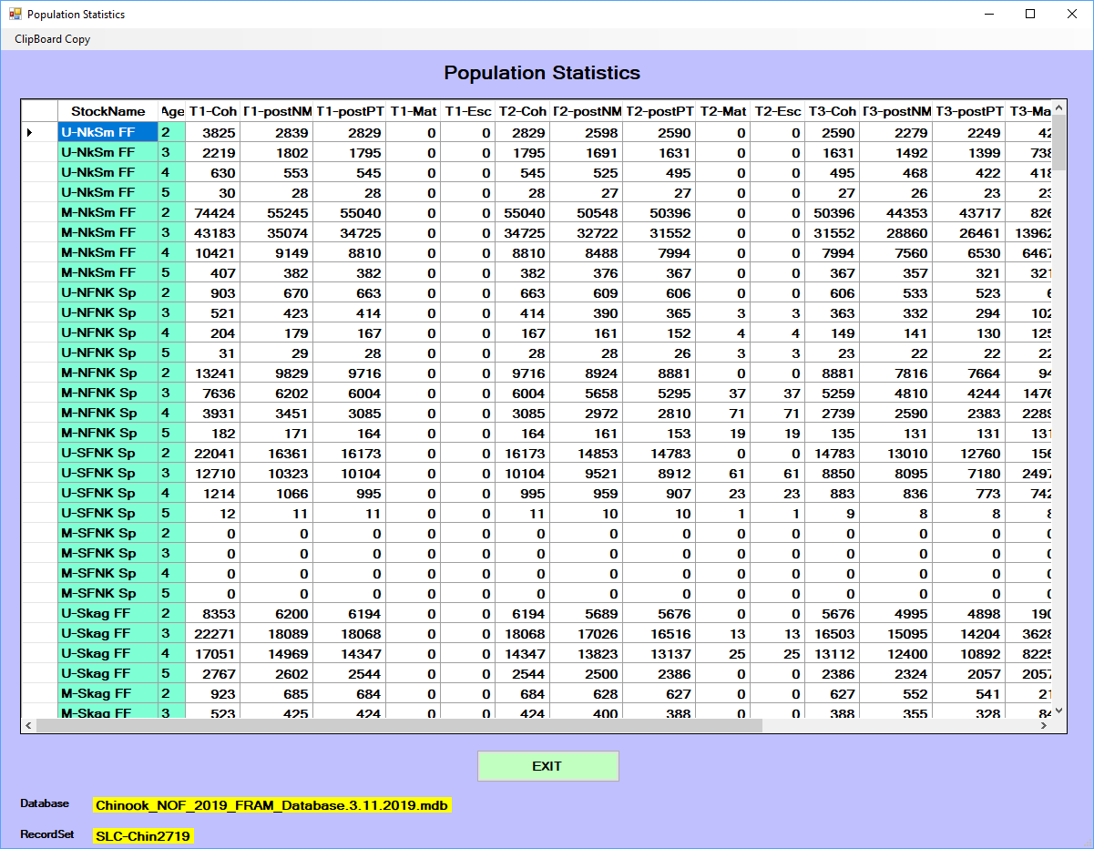
The “popstat” report is regularly used for Chinook, as it clearly
illustrates changes through the major FRAM processing
steps that take a stock from starting cohort to escapement. It presents
the cohort trajectory through time steps for each stock, broken out by
age for Chinook. The columns describe the progression through time of
the starting cohort through natural mortality, pre-terminal fisheries,
maturation, and terminal fisheries to escapement. For Chinook, note that
FRAM
currently calculates “marine escapement” while “spawning escapement” is
handled within TAMM.
For Chinook the report data represent by time step: starting cohort
by age (T#-StartCoh), cohort after natural mortality (T#-postNM), cohort
after pre-terminal fisheries (T#-postPT), mature cohort resulting from
stock-specific maturity age parameters as provided by the base period
(T#-Mat), escapement of the mature cohort remaining after FRAM’s set of
terminal fisheries (T#-Esc).

For Coho the report data represent by time step: starting cohort
(T#-Coht), cohort after natural mortality and pre-terminal fisheries
(T#-Rem), mature cohort in time step 5 (Oct-Dec) only (Mature), and
escapement of the mature cohort remaining after terminal and freshwater
fisheries (Escape; i.e. spawner escapement).

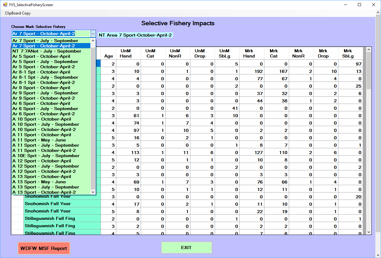
Mark-Selective Fishery Reports
This option generates detailed accounting of stock-specific mortality
for a selected mark-selective fishery and time step. All
fisheries/time-steps flagged as mark-selective in a particular model run
will be available in the drop-down menu on the upper left. Once a
selection is made, the values for each stock impacted in that
fishery/time-step are presented. Values for unmarked and marked
components include: handled fish, catch mortality, non-retention
mortality, drop-off mortality, and for Chinook only will include
sub-legal mortality.
Additionally, the red “WDFW
MSF Report” button
transfers Chinook information related to landings, encounters, and
mortalities aggregated across all stocks to an external Excel
spreadsheet. The button is not available for Coho modeling.

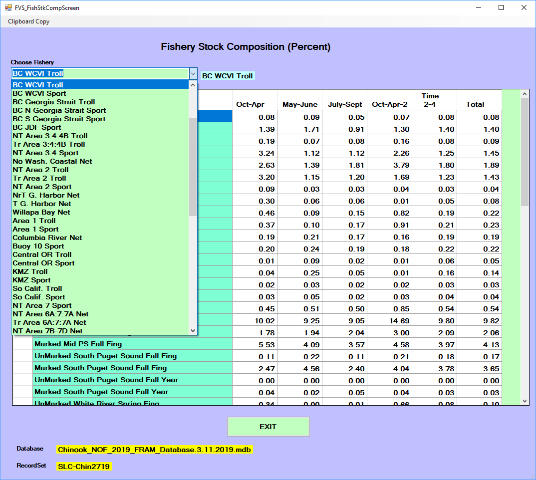
Fishery stock composition report
After selection of a single fishery from the drop-down menu, this
report displays the percentage of each stock within the total mortality
for each time step. Only those stocks impacted by the fishery will be
displayed (i.e. a different set of stocks can be displayed for each
fishery). Note: for Chinook fisheries without a 100% model stock
proportion, percentages within this report only represent the modeled
portion of the catch.

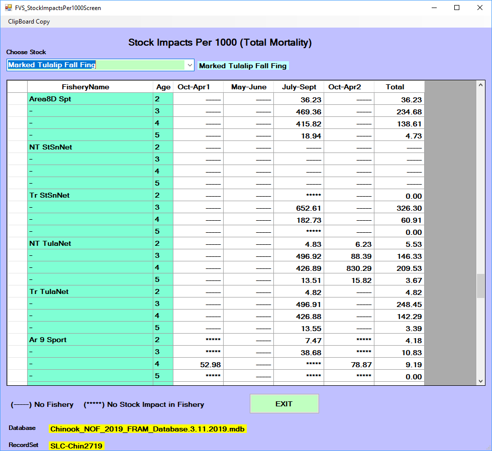
Stock impacts per 1000
This normalized view of stock-specific total mortality impacts for
each fishery and time step offers another perspective on relative
differences. This report demonstrates the stock contribution (in numbers
of non-AEQ fish) to a
hypothetical total mortality of 1,000 fish in each fishery/time step.
Only a single stock component can be selected (i.e. only the Skookum
Creek Hatchery Marked stock can be viewed and a separate selection would
be necessary to see the results for the Skookum Creek Hatchery Unmarked
stock).

Report Drivers
Report drivers generate 14 pre-formatted output report types using
unique instructions found in the report driver. Many of these reports
are also available as screen reports or found in FRAM output to
TAMM files. A
report driver is species-specific, tied to a unique base period for
parameters, and contains a header with metadata. The output reports are
given a .PRN file extension and can be opened with a text editor such as
Microsoft Notepad. The actual report drivers, with instructions on what
to include, are stored in the MS
Access project database table ReportDriver.
From the main menu, select “Output/Results”, “Report Driver File”, to
get to the report driver file options. The most straightforward step is
to “Select Driver” from the available report drivers already in the
project database table ReportDriver. Click the checkbox next to one from
the list and you will be re-directed back to the driver file options
menu. Next, click the “Run Reports” button to name and save the output
PRN file. Once you click save from
the prompt, the output PRN file is
generated and ready to view. The “Edit Report Driver” option is no
longer functional in updated versions of FRAM and thus a
new report driver must be created to make changes from an old one.
Changes to a report driver need to be made in the project database table
ReportDriver.
Many FRAM databases
include various previously created custom report drivers. To create a
new report driver, select “Output/Results”, “Report Driver File”,
“Create Report Driver”. Select the desired report from the 14 available
options and specify parameters for customization from the selection
boxes. A good example of a unique, customizable report is the “Terminal
Run Summary”. This report allows the user to specify fisheries and time
steps for inclusion in the terminal run definition of selected stocks.
When prompted, save the driver. The new driver will then appear in the
“Select Driver” report selection box. To produce output, select the new
driver and click “Run Report”.
TAMM
The current Terminal Area Management Module is a Microsoft Excel
spreadsheet that interfaces with the FRAM
application, providing additional input parameter values and receiving
outputs following a run.
The TAMMs
for Chinook and coho differ in most details, but both share a general
conceptual division into sheets related to FRAM inputs,
those compiling FRAM outputs,
and then those that draw from these first two classes to perform
numerous additional calculations and manipulations associated with
particular tabular report breakouts. Regional areas in Puget Sound are
also represented within individual sheets to customize output for
regional management perspectives. In addition, a Documentation sheet
notes modifications and/or revisions made to the TAMM file or
structure overall (e.g. a formula error was fixed or a new section was
added), and a RunLog sheet notates model input changes between model
runs during an annual preseason planning process.
For preseason runs, the typical naming convention follows a pattern
of “specNNYY”, with “Chin” or “Coho” followed by an “comanager agreed”
run number and the 2-digit year. For example, the final 2019 Chinnok
model run was “Chin2719” while the coho file was “Coho1925”.
Note that the TAMM files contain
historical information, including outdated tables or sheets. Over the
years, perspectives and technical approaches have changed and yet the
older pages or sections remain. Preserving these historical approaches
in case they are needed again, while adding new or updating content can
create confusion about which content is maintained and relevant. Some
completely obsolete sheets are hidden using Excel and an attempt is made
to hide columns or sections of sheets that are no longer used.
Running FRAM with TAMM
Note: An “official” FRAM run should
always be run with a TAMM!
TAMM is
rooted in the management history of Puget Sound Chinook and Coho salmon.
Prior to the existence of FRAM,
spreadsheet models calculated terminal fisheries’ impacts with ‘simple
harvest rates’. A harvest rate is computed as terminal catch divided by
terminal abundance. Abundance accounting occurred in run reconstruction
spreadsheets that calculated terminal abundance as escapement +
freshwater landed catch + terminal landed catch. FRAM introduced
the ability to calculate stock specific impacts in mixed stock
pre-terminal areas using exploitation rates. Exploitation rates are
computed as catch of a stock divided by the abundance of the stock.
Whereas harvest rates are area-specific, exploitation rates are
stock-specific. Using harvest rates in terminal areas with typically
very low proportions of non-local stocks introduced an acceptable
amounts of error, while providing the convenience of simple
calculations.
The practice of computing harvest rates in terminal and extreme
terminal fisheries continues to this day. Unfortunately, it is
incompatible with FRAM
exploitation rate calculations. TAMM reports
terminal harvest rates to FRAM. FRAM translates
these harvest rates into exploitation rates through an iterative
process. FRAM uses
instructions about the stock/fishery make-up of the terminal area in
order to reconstruct the denominator of the original harvest rate
calculation. Given these denominators, the model calculates landed
catches and associated fishery scalers. FRAM also
computes non-local stock impacts in terminal areas. Landed catches and
fishery scalers are saved to the model run database.
Upon selecting to “Run Model” a submenu presents the user with the
option to “Select TAMM”. If this
option is chosen, a file selection dialogue box appears. Select the
desired TAMM
and click “Open”. After FRAM completes
iterations, the following message box pops up, and selecting “Yes”
results in FRAM importing
output into the TAMX for Chinook or PRN Sheets for Coho. Note that although values
are imported, they are not yet saved and require standard Excel saving
procedures.
There are two primary reasons to run a FRAM model
with a TAMM file. Although
these reasons often apply, it is acceptable to run FRAM without
TAMM if they
do not. This can speed up the time it takes to perform a Chinook model
run. However there can be interactions between input into FRAM (from
TAMI) and outputs from FRAM into TAMM so that it may
take more than one iteration of cycling FRAM output
back into TAMM, before TAMI
values stabilize. This is especially noteworthy for runs with
significant abundance and /or fishery changes.
- TAMM
input is needed
FRAM has not
been run with a TAMM file before or
sheet TAMI and/or FRAM inputs
have changed since the model was last run with a TAMM file. Once
FRAM runs
with a TAMM
file, static input values for TAMM fisheries are
stored in the FRAM project
database. For Chinook, when the model is run a second time, a TAMM may not be
needed to reproduce the model run results from the first run with a
TAMM
file.
However, there are some TAMI fishery inputs in the coho TAMM, which are
dependent on model results of terminal run size to subsequently update
the input value when other fishery inputs are modified. This type of
iteration is not built into the software for Puget Sound fisheries and
thus the TAMM
file is dynamic in terms of updating terminal fishery inputs. The coho
TAMM is also
used for WA coastal terminal
fisheries, which utilize a selected button to run built-in software
iterations which update input values that are dependent on model results
of terminal run size.
- TAMM
output is needed
Chinook: FRAM contains
pre-terminal and terminal fisheries, but does not account for freshwater
fisheries or escapements; both of which are only contained within the
TAMM file
structure. FRAM also does
not provide exploitation rates or the breakdown of stock components to
align with conservation management objectives. Thus, running a model
with the TAMM
file is necessary to generate the full suite of fishery impacts and
stock breakdown to calculate and assess management.
Coho: FRAM contains
pre-terminal, terminal, and freshwater fisheries as well as escapement.
However, FRAM does not
provide exploitation rates or the aggregation of stock components to
align with conservation management objectives. Thus, running a model
with the TAMM
file can provide calculation of exploitation rates and values aligned
with conservation management objectives. Coho TAMM outputs are
also needed by other external models that in turn relay revised inputs
back to the FRAM/TAMM modeling
framework (i.e. TAMM output values
are used as input values in WA coast
terminal area regional models and in Columbia River models).
Coho TAMM
This tool is used to:
- provide fishery inputs to FRAM from Puget
Sound and Washington coastal terminal areas,
- calculate exploitation rates (ERs), and
- summarize model output to evaluate achievement of management
objectives.
Many sheets in the Coho TAMM workbook
involve post-processing calculations and formatted reporting. The
sections below focus on a subset of sheets likely to be the focus of the
majority of user interactions.
Coho TAMM
sends to FRAM: - Tami
sheet – contains FRAM inputs; a
precursor sheet with more details about Tami values is Input_Harvestnew
- WACoastTerminal – contains FRAM inputs
when using “Run Coastal Iterations”
Coho FRAM sends back
to TAMM: -
FishSumAllPRN, Table2PRN, StockSumPRN, TRunsPRN – FRAM output in
terms of all stocks/fisheries.
Tami
The Tami sheet compiles values from the Input_Harvestnew sheet and
passes them to FRAM. A
separate flagging system is used in the Coho Tami sheet to depict each
type of fishery input: flag 1 = catch, flag 2 = effort scalar, 3 = TAA harvest rate, 4 = ETRS
harvest rate. A flag value of -99 tells FRAM to ignore
TAMM inputs
and to use the inputs provided within the FRAM
interface/database.
The Tami sheet also contains information needed for harvest rate
iteration calculations. Fishery harvest rate inputs are provided with a
specific definition of how that rate was calculated, so that FRAM can apply
it correctly. A numeric system is used to represent these definitions
and are stored in the Coho FRAM project
database table “TAAETRSList”. The numeric value for which harvest rate
definition is associated with the fishery input is provided on the Tami
sheet under Abundance Definitions. In general, the TAA rates are calculated
with total catch while the ETRS rates only include
catch of local stocks.
WACoastTerminal
The WACoastTerminal sheet is used ensure that FRAM’s catch
composition of local stocks in Washington coastal terminal fisheries
(per base period and time step) are consistent with the stock catch
composition derived with regional harvest management planning models.
Stock-specific harvest rates from regional harvest management models are
input into the WACoastTerminal sheet. These rates are applied against
the stock’s terminal run size from FRAM output.
The FRAM
ratio of local to non-local stocks is used to then calculate a total
catch for each terminal fishery, which is apportioned to time step based
on regional models. These catch inputs are then summarized into a
formatted table in the lower section of the sheet and read back into
FRAM
using the FRAM model run
specification button “Run Coastal Iterations”.
Within this sheet, a fishery flag value of -99 tells FRAM to ignore
TAMM inputs
using the local stock-specific harvest rates and base subsequent
calculations for evaluating management on the FRAM catch
composition only (per base period and time step). For preseason
planning, a fishery flag of -88 is used in the sheet so that subsequent
calculations for evaluating management utilize the resulting stock catch
composition consistent with the regional harvest management planning
models.
PRN Sheets
There are four “PRN” sheets in the Coho TAMM file, which
are created by driver files (.DRV) as defined in the coho FRAM project
database table “ReportDriver”. These provide direct output of model
results from each FRAM model run.
Hyperlinks to individual sections within the sheet are found in the
upper right section, and the key strokes Control+Home can be used to
return to the top of the sheet. The four “PRN” sheets are as
follows:
- FishSumAllPRN – Generated by FisherySummaryAllMortalities.DRV
definitions. Summarizes impacts for all Coho stocks in each fishery and
time step. These include sections for a.) landed catch, b.) shaker
mortality (drop-off and drop-out mortalities), c.) non-retention
mortality (CNR inputs and mark-selective release mortalities), d.)
landed catch plus non-retention mortality, e.) total mortality.
- StockSumAllPRN – Generated by CohoStockSummary.DRV definitions.
Reports total mortality by stock (marked and unmarked) summed over all
fisheries and time steps.
- Table2PRN – Generated by PSCTable2.DRV definitions. Reports total
mortality for a specified stock or stock aggregate by time step. There
is also a configured section for verifying stock-specific fishery rate
scalars for the non-treaty and treaty Area 8D net fisheries impacts on
marked stocks.
- TRunsPRN – Generated by PSCTRuns.DRV definitions. For aggregates of
various fisheries or stocks, reports values for a.) terminal run size,
b.) escapement, and c.) terminal run size with all mortality for stock
aggregates.
Sheet “2”
This sheet contains multiple tables for Coho fishery impact summary
highlights. Total fishery related mortality is presented for aggregated
fisheries and stocks. Various statistics are calculated and compared to
management guidelines. These are dependent upon stock and regional
management approaches. Table format differs for Puget Sound, Washington
coast, and hatchery stocks summaries.
Sheet “4”
This sheet contains a summary table of Coho exploitation rates by
fishery aggregate for key Puget Sound and Washington natural stocks.
Rates are calculated for ocean exploitation, Puget Sound exploitation,
total exploitation, and southern US exploitation. In addition, treaty
and non-treaty rates are presented as sub-categories.
Overview of Coho TAMM workbook
sheets
|
Table
|
Description
|
|
1
|
Table 1: Description of fishery regulations & summary of Coho catch
quotas/targets (**Comments/Descriptions should be updated each year)
|
|
2
|
Table 2A,2B,2C,2D,2E: Coho fishery impact summary highlights
(**Management Objectives may be updated each year)
|
|
4
|
Table 4: Summary of Coho exploitation rates by fishery aggregate
|
|
7
|
Table 7: Coho run sizes for Pacific Fishery Management Council (PFMC)
Salmon Technical Team (STT) reference
|
|
Sk
|
Skagit region impact calculations/summaries
|
|
StSn
|
Stillaguamish-Snohomish region impact calculations/summaries
|
|
HdC
|
Hood Canal region impact calculations/summaries
|
|
SPS
|
South & Mid Puget Sound impact calculations/summaries
|
|
NS
|
Nooksack-Samish region impact calculations/summaries
|
|
JDF
|
Juan de Fuca region impact calculations/summaries
|
|
PFMCTable7
|
Pacific Fishery Management Council (PFMC) Table 7 (Supplemental STT
Reports/Preseason Report II and III); tracking LCN, OCN, RK
|
|
WACoastTerminal
|
Tables related to WA coastal terminal fisheries/areas, including
generation of FRAM fishery inputs
|
|
Thompson
|
Table T: Thompson and Upper Fraser Coho fishery impact summary
|
|
Input_Harvestnew
|
Location where Fishery inputs are entered for TAMM terminal and extreme
terminal net & sport fisheries
|
|
Tami
|
TAMM user Inputs transferred from TAMM to FRAM
|
|
FishSumAllPRN
|
FRAM outputs transferred from FRAM to TAMM: Fishery Summary
|
|
Table2PRN
|
FRAM outputs transferred from FRAM to TAMM: Stock Catch Summary (uses
PSCTable2.drv)
|
|
StockSumPRN
|
FRAM outputs transferred from FRAM to TAMM: Stock Summary
|
|
TRunsPRN
|
FRAM outputs transferred from FRAM to TAMM: Terminal Run Report (uses
PSCTRuns.drv)
|
|
LandedCNRTMbyTP
|
Pacific Fishery Management Council (PFMC), Salmon Technical Team use for
reporting and table values (Annual Review of Fisheries, Preseason
Reports)
|
|
FisheryConvTemplate
|
Original template based on older version of FRAM, for PFMC STT reporting
and table values (see LandedCNRTMbyTP in use now)
|
|
NT-Tsummary
|
Treaty and non-treaty allocation summary by Puget Sound management unit
aggregates
|
|
PS_HatcheryEsc.
|
Table H. Hatchery escapement to Puget Sound broodstock collection
facilities (**Should be updated each year)
|
|
Documentation
|
Modifications and/or revisions made to the TAMM structure or file
overall (See RunLog for specific model input changes)
|
|
fram_unm_mrkprn
|
Intermediate calculation page for Columbia River FRAM outputs, used by
PFMC STT
|
|
FramScalarsOPIstyle
|
Source: OPITT, (provided in February for preseason planning)
|
|
ColR&OCN&RogKlam
|
Source: OPITT, (provided in February for preseason planning)
|
|
ColRPercent
|
Source: OPITT, related to Columbia River, used by PFMC STT
|
|
ColRHarvestInput
|
Source: OPITT, related to Columbia River, used by PFMC STT
|
|
AttachC
|
Source: OPITT, related to Columbia River, used by PFMC STT
|
|
AttachCStkInput
|
Source: OPITT, related to Columbia River, used by PFMC STT
|
|
SportMatrix
|
Regulation summary for Puget Sound marine sport by fishery and model
time periods (Source: WDFW; **Should be updated each year or with
changes between model runs)
|
|
RunLog
|
Notation of model input changes between model runs (See Documentation
for file/format revisions)
|
|
Preseason_Tracking
|
Tracking of model runs as preseason planning progresses, with relevant
file and model run descriptions
|
|
CohoStock_Reference
|
For Reference. Source: 2018PFMC_NOF_CohoFRAMdatabase_Draft.mdb; Table:
Stock (Species=COHO)
|
|
CohoFishery_Reference
|
For Reference. Source: 2018PFMC_NOF_CohoFRAMdatabase_Draft.mdb; Table:
Fishery (Species=COHO)
|
|
TAAETRSList_Reference
|
For reference. Source: CohoPugetSound2019TAMMInputTemplate_MB012819.xlsx
(MB)
|
Chinook TAMM
This tool is used to:
- split stocks that are aggregated in FRAM into finer
sub-components
- account for fisheries that are not in FRAM
- calculate exploitation rates (ERs) and escapements over several
levels of stock detail
Many sheets in the Chinook workbook involve post-processing
calculations and reporting, with similar (but not identical) layout and
related content. The sections below focus on the smaller group of sheets
likely to be the focus of the majority of user interactions.
Chinook TAMM passes values
in the sheet TAMI to FRAM, and
subsequently receives FRAM output
compiled in the sheet TAMX.
FRAM-TAMM stock
lookup
Several FRAM stock
aggregates are broken out in TAMM.
Stock units in FRAM and TAMM
|
Region
|
FRAM
|
TAMM
|
|
HOOD CANAL
|
Hood Canal Fingerling
|
Area 12B tribs natural
|
|
HOOD CANAL
|
Hood Canal Fingerling
|
Hoodsport Fi
|
|
HOOD CANAL
|
Hood Canal Fingerling
|
Skokomish R. nat
|
|
HOOD CANAL
|
Hood Canal Fingerling
|
Skokomish R. hatchery
|
|
HOOD CANAL
|
Hood Canal Fingerling
|
Area 12C-D tribs natural
|
|
HOOD CANAL
|
Hood Canal Yearling
|
Hoodsport Yr
|
|
JDF
|
Elwha/Dungness
|
Dungeness
|
|
JDF
|
Elwha/Dungness
|
Elwha
|
|
JDF
|
Hoko
|
Hoko
|
|
NOOKSACK/SAMISH
|
Nooksack/Samish S/F
|
7E Glenwood Springs hatchery
|
|
NOOKSACK/SAMISH
|
Nooksack/Samish S/F
|
Lummi Bay hatchery
|
|
NOOKSACK/SAMISH
|
Nooksack/Samish S/F
|
Samish R. hatchery
|
|
NOOKSACK/SAMISH
|
Nooksack/Samish S/F
|
Samish R. natural
|
|
NOOKSACK/SAMISH
|
North Fork & South Fork Nook Spring (2)
|
Nooksack Early
|
|
SKAGIT
|
Skag S/F Fi
|
Skag S/F Fi
|
|
SKAGIT
|
Skagit S/F Yr
|
Skagit S/F Yr
|
|
SKAGIT
|
Skagit Spr
|
Skagit Spr
|
|
SOUTH SOUND
|
Deep SPS Fingerlings
|
Carr Inlet/Minter Hatchery
|
|
SOUTH SOUND
|
Deep SPS Fingerlings
|
Carr Inlet/Minter Nat
|
|
SOUTH SOUND
|
Deep SPS Fingerlings
|
Chambers Creek Hatchery Fing
|
|
SOUTH SOUND
|
Deep SPS Fingerlings
|
Nisqually River Hatchery
|
|
SOUTH SOUND
|
Deep SPS Fingerlings
|
Nisqually River Nat
|
|
SOUTH SOUND
|
Deep SPS Fingerlings
|
McAllister Creek Hatchery
|
|
SOUTH SOUND
|
Deep SPS Fingerlings
|
McAllister Creek Nat
|
|
SOUTH SOUND
|
Deep SPS Fingerlings
|
Deschutes/Cap. Lake Hatchery
|
|
SOUTH SOUND
|
SPS Yearlings
|
Duwamish-Green Yearlings
|
|
SOUTH SOUND
|
SPS Yearlings
|
Carr Inlet Minter Yearlings
|
|
SOUTH SOUND
|
SPS Yearlings
|
Chambers Creek Yearlings
|
|
SOUTH SOUND
|
SPS Yearlings
|
Deschutes Cap. Yearlings
|
|
SOUTH SOUND
|
Upper SPS Fingerlings
|
Grovers Ck. Hat. - 10
|
|
SOUTH SOUND
|
Upper SPS Fingerlings
|
Lk. Washington Hatchery
|
|
SOUTH SOUND
|
Upper SPS Fingerlings
|
Lk WashingtonNatural
|
|
SOUTH SOUND
|
Upper SPS Fingerlings
|
Duwamish-Green Hatchery
|
|
SOUTH SOUND
|
Upper SPS Fingerlings
|
Duwamish-Green Nat
|
|
SOUTH SOUND
|
Upper SPS Fingerlings
|
Gorst Creek Hat. - 10E
|
|
SOUTH SOUND
|
Upper SPS Fingerlings
|
Gorst Creek Yearlings
|
|
SOUTH SOUND
|
Upper SPS Fingerlings
|
Puyallup River Hatchery
|
|
SOUTH SOUND
|
Upper SPS Fingerlings
|
Puyallup River Nat
|
|
SOUTH SOUND
|
UW Accelerated
|
UWAcc
|
|
STILLAGUAMISH/SNOHOMISH
|
Sno S/F Fi
|
Sno S/F Fi
|
|
STILLAGUAMISH/SNOHOMISH
|
Sno S/F Yr
|
Sno S/F Yr
|
|
STILLAGUAMISH/SNOHOMISH
|
Stilly S/F
|
Stilly S/F
|
|
STILLAGUAMISH/SNOHOMISH
|
Tulalip Hatchery
|
Tulalip Hatchery
|
TAMI
The TAMI sheet passes in values for several fisheries. A flag value
of -88 tells FRAM to ignore
TAMM inputs
and to use the inputs provided within the FRAM
database.
Additional flags determine whether the parameter values are
interpreted as a rate or count (i.e., number of fish), with the values
themselves derived from Input Page entries and
additional calculations on area-specific sheets.
For example, in the screenshot shown above, the Bellingham Bay values
that are sent to FRAMM first pass through the “NS” Nooksack-Samish sheet
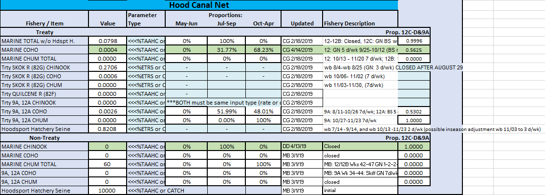
from the block of input page cells denoted “Rate” is %TAA
Nooksack-Samish Aggregate Summer/Fall chinook.
- 7BCD NT
- C8 May-Jun: “0.0000” =IF(+NS!Y17=“na”,0,NS!Y17) <- NS!Y17 hard
entered
- D8 Jul-Sep: “0.1571” =NS!Z17 <- NS!P20 <- Input Page!B221
<- derived from B’ham Bay purse seine and gillnet mortality data
- E8 Oct-Apr: “19” =NS!AA17 <- NS!P22 <- Input Page!B223 <-
as for summer timestep
- J8 EQADJ: “0” =NS!AC23 <- NS!P38 <- Input Page!B226 <-
currently unused
- 7BCD Treaty
- C9 May-Jun: “0” =NS!Y18 <- NS!P19 <- Input Page!B220 <-
based on planned treaty harvest
- D9 Jul-Sep: “0.2892” =NS!Z18 <- NS!P21 <- Input Page!B222
<- as for spring timestep
- E9 Oct-Apr: “0.001” =NS!AA18 <- NS!P23 <- Input Page!B224
<- as for spring timestep
As general good practice, after making any changes to TAMM fishery
parameters, particularly those that are passed to and processed within
FRAM, it
may be worthwhile to ensure that the intended behavior occurred by
checking relevant screen reports and/or TAMM output
sheets.
Input Page
This sheet is divided (row-wise) into sections for stock forecasts,
net fisheries, and sport fisheries, with each of these primary sections
further subdivided by river basins. Note that in addition to the text
descriptions, hover/tooltip Excel comments are associated with several
cells and can provide greater context.
During the pre-season process, values are agreed-to stock forecasts
and anticipated fisheries from regional co-managers.
When performing post-season runs, the values are agreed-to abundance
estimates from regional co-managers and observed fishery catches from
co-manager technical staff.
In general, across areas, the counts of hatchery marked, hatchery
unmarked, natural marked and natural unmarked returns are provided for
the different stock components.
Skagit
- HM/HUM/NM/NUM are provided for spring, S/F fingerling & S/F
yearling (these values are used to derive proportions for
recruit scalers?)
- The summer/fall run is further divided into Upper Skagit Summer,
Lower Sauk Summer, and Lower Skagit Fall
- The spring run is divided into Upper Sauk Spring, Suiattle Spring,
and Upper Cascade Spring

- Treaty impacts are entered for:
- marine Chinook, sockeye, pink, coho, chum, steelhead and test
fisheries
- freshwater Chinook, C&S, sockeye, pink, coho, chum, steelhead
and test fisheries
- Non-treaty (incidental) impacts are entered for pink and chum
fisheries

- Incidental impacts are entered for the sport coho and sockeye
fisheries
- Mark-selective (MSF) parameters are entered
for the impacts on Springs

Stillaguamish & Snohomish
- HM/HUM/NM/NUM are provided for Snohomish S/F fingerlings and
yearlings, Stillaguamish S/F, and Tulalip hatchery fish
- The Skykomish portion of the Snohomish naturals is entered

- Treaty impacts are entered for
- Area 8A C&S, coho, chum, steelhead and test fisheries
- Stillaguamish C&S, pink, coho and chum fisheries
- Snohomish River commercial
- Area 8D coho
- Non-treaty (incidental) impacts are entered for Area 8D and Area 8A
pink, coho and chum fisheries

- Catches are entered for Stillaguamish and Snohomish Rivers
- Mark-selective (MSF) parameters are entered for the Skykomish
River

Hood Canal
- HM/HUM/NM/NUM are provided for Area 12B tribs natural, Hoodsport
hatchery fingerlings and yearlings, Skokomish natural and hatchery, and
Area 12C-D tribs natural fish

- Treaty impacts from marine coho and chum and in-river Chinook are
entered by season (May-Jun, Jul-Sep, Oct-Apr)
- Non-treaty impacts from coho and chum fisheries are entered by
season along with the Hoodsport hatchery beach seine catch

- Catches are entered for the Quilcene and miscellaneous 12 B/C/D
fisheries
- Mark-selective (MSF) parameters are entered
for the Skokomish River

South Puget Sound
- HM/HUM/NM/NUM are provided for Grovers Creek hatchery, Lake
Washington hatchery and natural, Sammamish natural, Duwamish-Green
hatchery and natural, Gorst Creek hatchery, Puyallup River hatchery and
natural, Carr Inlet/Minter hatchery and natural, Chambers Creek
hatchery, Nisqually River hatchery and natural, McAllister Creek
hatchery and natural, Deschutes River hatchery, miscellaneous
13D-K/Coulter Creek hatchery, and White River natural and hatchery
- The marked/unmarked yearlings are listed for the Duwamish and White
River components
- Proportions are entered for several hatchery stocks that spawn in
river and the proportion of “natural” returning to the hatchery

- Harvest rates are entered for the 11A, Puyallup River and White
River C&S impacts on the White River spring run
- Terminal/near-terminal marine catches by season (May-Jun, Jul-Sep,
Oct-Apr) are entered for
- Area 10/11 treaty and non-treaty commercial (incidental in chum
fishery)
- test fisheries
- Area 10A treaty, C&S, and non-treaty
- Area 10E treaty and non-treaty
- Area 13/13D-K/13A treaty and non-treaty
- Freshwater treaty net and C&S impacts are entered for Lake
Washington, Lake Sammamish, the Duwamish-Green River, the Puyallup
River, the Nisqually River, and McAllister, Minter and Chambers Creeks
- Mark-selective parameters are also entered for the Nisqually tangle
net fishery

- Catches are entered for Lake Washington, Lake Sammamish, the
Duwamish-Green River, McAllister Creek, Minter Creek, Chambers Creek,
Deschutes/Capital Lake and Kennedy/misc 13B
- Mark-selective (MSF) parameters are entered
for fisheries in Puyallup, Carbon and Nisqually Rivers

Nooksack & Samish
- HM/HUM/NM/NUM are provided for Nooksack Early (Spring) hatchery and
natural, Glenwood hatchery, Lummi Bay hatchery, and Samish River
hatchery and natural
- The proportion of North Fork natural origin fish in the total
natural origin fish is entered

- Nooksack spring/early impacts are entered for C&S fisheries as
catches or harvest rates
- Mark-selective parameters are also entered for the Lummi tangle net
fishery
- Nooksack summer/fall impacts for treaty and non-treaty fisheries are
entered by season (May-Jun, Jul-Sep, Oct-Apr)

- Catches for the Samish/Whatcom sport fishery and Nooksack River
MSF can be entered
- the MSF includes
marked-release and unmarked retention parameter values

Strait of Juan de Fuca
- HM/HUM/NM/NUM are provided for Dungeness, Elwha, and Hoko runs
- pre-spawn mortality is entered for Dungeness and Elwha

- Catches can be entered for Dungeness Bay treaty and non-treaty net
fisheries, for Elwha C&S and test/commercial, and for Hoko terminal
and extreme terminal fisheries

- Sport fishery catches can be entered for Dungeness, Elwha, and
Hoko

TAMX
During a run with a Chinook TAMM selected,
FRAM
passes output values to the TAMX sheet. Generally, these are organized
into row-wise blocks of fisheries by stock after a header block of all
stocks summed across fisheries.
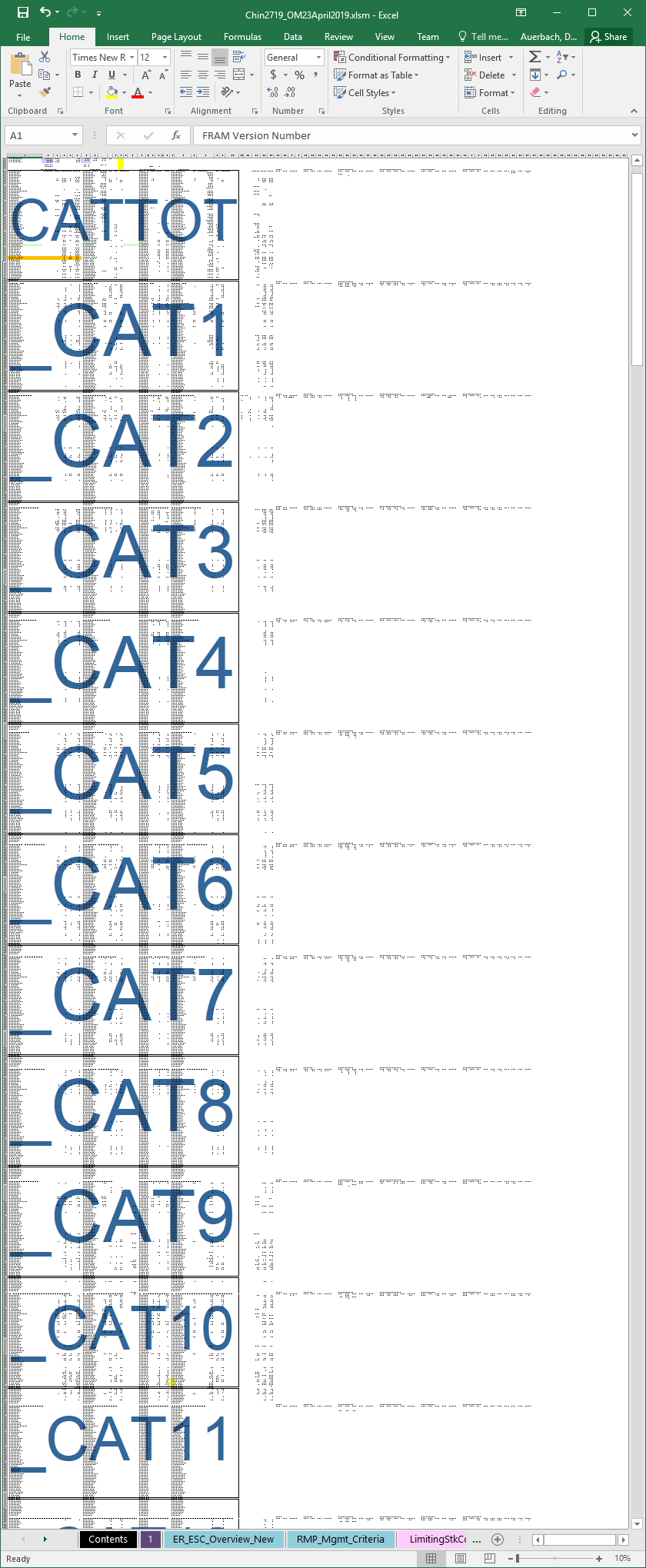
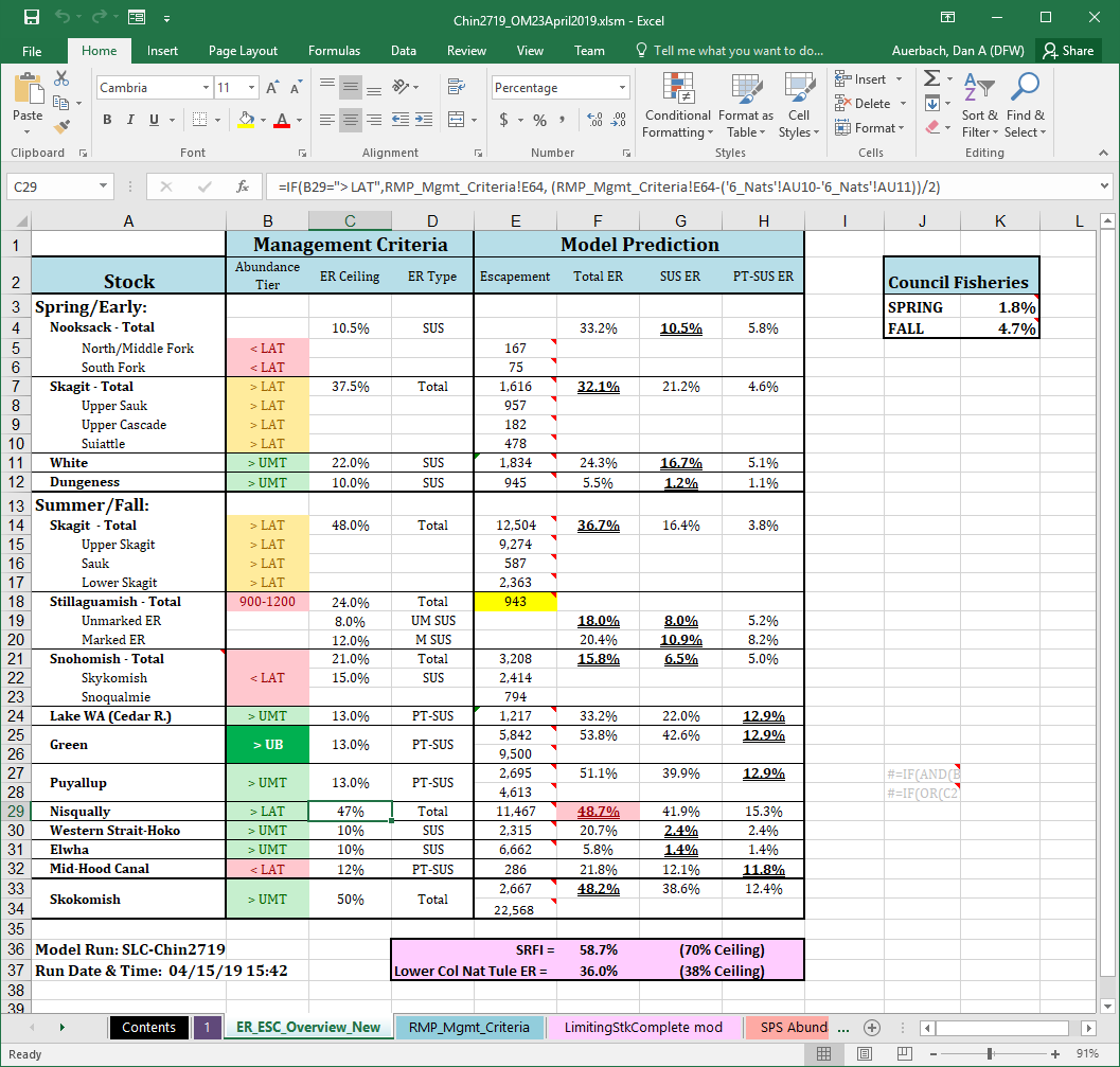
ER_ESC_Overview_New
The exploitation rate and escapement overview approximates a primary
“dashboard” of ESA
compliance for the Washington comanagers, displaying estimated
exploitation rates and escapements relative to the critical thresholds
defined in stock-specific management unit plans (which are also listed
in the RMP_Mgmt_Criteria sheet).
Conditional formatting indicates stocks with exploitation rates
exceeding management targets. In pre-season runs, this indicates that
fishery adjustments will be necessary to meet management objectives. In
post-season runs, this indicates that the stock failed management
objectives, given fisheries and abundances that actually occurred.
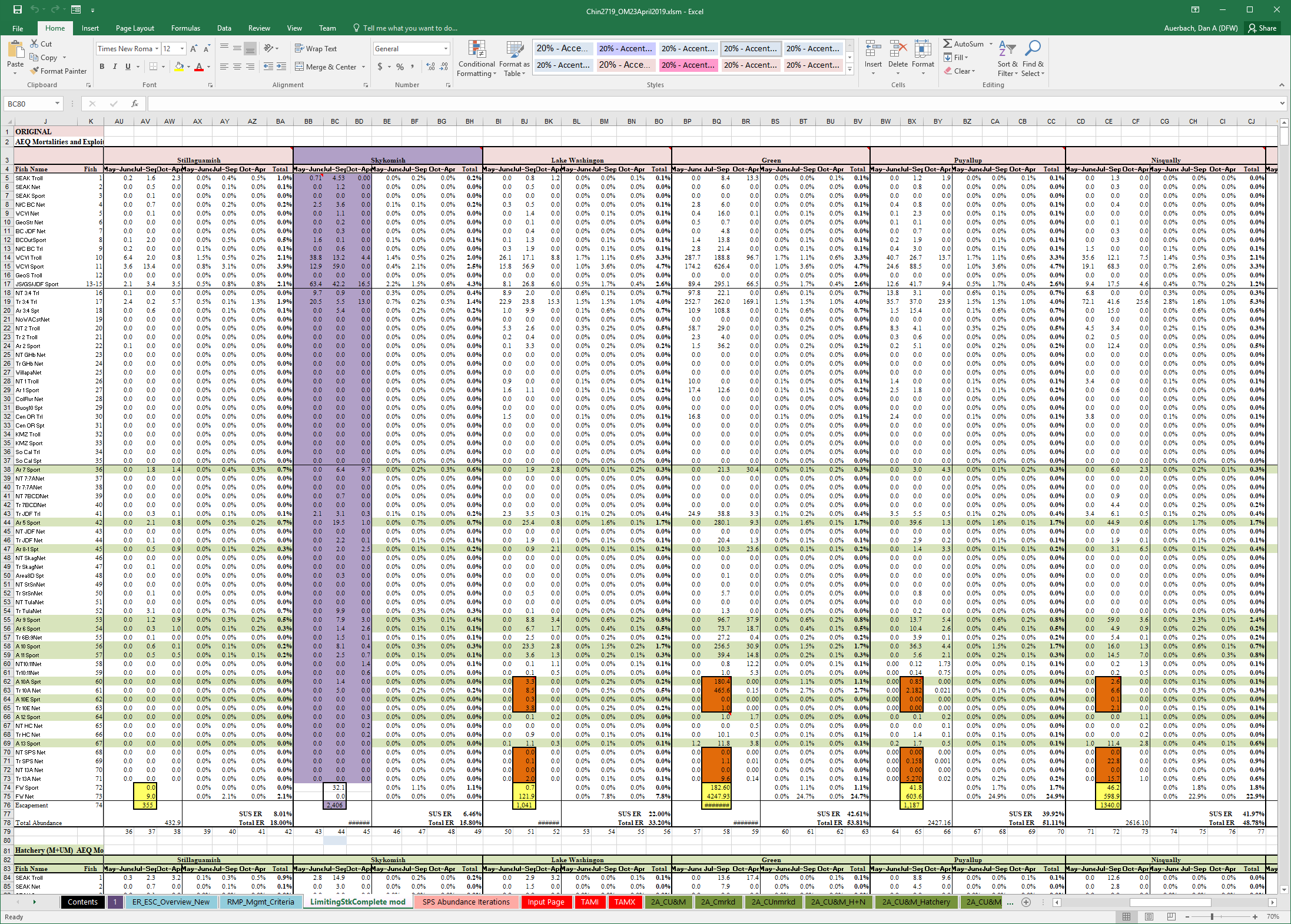
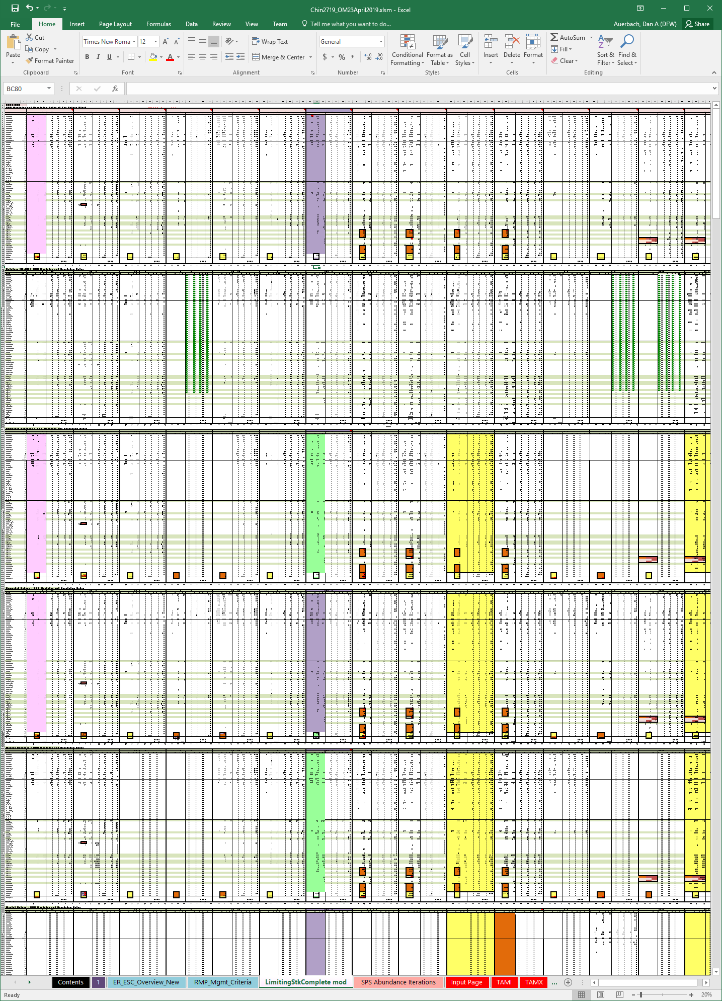
LimitingStock
This sheet offers similar information to that found in the overview,
but with greater detail on the particular breakdown of impacts to stocks
within specific fisheries. It consists of blocks of values for:
- “Original” key natural stocks
- Hatchery (M+UM)
- Unmarked hatchery
- Unmarked natural
- Marked hatchery
- Marked natural
The LimitingStock table is a great source of information for
technical staff interested in better understanding which fishery-time
steps have the greatest estimated impact on a stock within a given
year.
Overview of Chinook TAMM workbook
sheets
|
Table
|
Description
|
|
1
|
Table 1: Description of fishery regulations & summary of Chinook
catch quotas/targets
|
|
ER_ESC_Overview(ifanyMSF)
|
Impact summary for ESA-listed stocks (total, SUS, and SUS PT ERs;
natural escapements); aka "Table 2"
|
|
LimitingStkComplete mod
|
Detailed (fishery-by-fishery) impact distribution for constraining
stocks
|
|
SPS Abundance Iterations
|
Complete this worksheet to properly adjust SPS abundances based on
stock-specific catches in the SPS terminal net fisheries
|
|
Input Page
|
Location where (1) Stock, (2) Net Fishery, and (3) Sport Fishery are
entered for TAMM stocks
|
|
TAMI
|
TAMM user Inputs transferred from TAMM to FRAM
|
|
TAMX
|
FRAM outputs transferred from FRAM to TAMM
|
|
2A_CU&M
|
Disaggregated stock impacts (FRAM stock split into TAMM stocks) by FRAM
fishery and TAMM freshwater fishery for MARKED & UNMARKED fish;
built off of 2D_Fmrkd, 2D_Funmrkd and stock worksheets
|
|
2A_Cmrkd
|
Similar to 2A_CU&M but for MARKED only
|
|
2A_CUnmrkd
|
Similar to 2A_CU&M but for UNMARKED only
|
|
2A_CU&M_H+N
|
Similar to 2A_CU&M, but now includes missing hatchery components for
Skagit and Stilly/Sno
|
|
2A_CU&M_Hatchery
|
Similar to 2A_CU&M, but only includes hatchery components for TAMM
stocks
|
|
2A_CU&M_N
|
Similar to 2A_CU&M, but only includes natural components for TAMM
stocks; generally computed as difference between 2A_CU&M H+N and
2A_CU&M Hatchery
|
|
2D_F
|
Total AEQ Mortalities and Landed Catch for MARKED and UnMARKED stocks by
fishery, less freshwater fishery impacts
|
|
2D_Fmrkd
|
Total AEQ Mortalities and Landed Catch for MARKED stocks by fishery,
less freshwater fishery impacts
|
|
2D_FUnmrkd
|
Total AEQ Mortalities and Landed Catch for UNMARKED stocks by fishery,
less freshwater fishery impacts
|
|
3
|
Table 3: Approximate allocation accounting
|
|
5
|
Table 5: Summary of exploitation rates by fishery aggregate
|
|
5_U&M
|
Table 5: Summary of exploitation rates by fishery aggregate
|
|
5Unmrkd
|
Table 5: Summary of exploitation rates by fishery aggregate, UNMARKED
Only
|
|
6
|
Table 6: Chinook ERs and mortality distribution by fishery aggregate
(MARKED + UNMARKED, HATCH. + NAT.)
|
|
6_U&M
|
Table 6: Chinook ERs and mortality distribution by fishery aggregate
|
|
6_Nats
|
Table 6: Chinook ERs and mortality distribution by fishery aggregate,
NATURAL ONLY
|
|
6Unmrkd
|
Table 6: Chinook ERs and mortality distribution by fishery aggregate
|
|
Sk
|
Skagit sp, su/fa impact calculations/summaries
|
|
Skmrkd
|
Skagit-MARKED sp, su/fa impact calculations/summaries
|
|
SkUnmrkd
|
Skagit-UNMARKED sp, su/fa impact calculations/summaries
|
|
StSn
|
Stillaguamish-Snohomish impact calculations/summaries
|
|
StSnmrkd
|
Stillaguamish-Snohomish-MARKED sp, su/fa impact calculations/summaries
|
|
StSnUnmrkd
|
Stillaguamish-Snohomish-UNMARKED sp, su/fa impact calculations/summaries
|
|
HdC
|
Hood Canal impact calculations/summaries
|
|
HdCmrkd
|
Hood Canal-MARKED sp, su/fa impact calculations/summaries
|
|
HdCUnmrkd
|
Hood Canal -UNMARKED sp, su/fa impact calculations/summaries
|
|
SPS
|
South & Mid Puget Sound impact calculations/summaries
|
|
SPSmrkd
|
South & Mid Puget Sound-MARKED sp, su/fa impact
calculations/summaries
|
|
SPSUnmrkd
|
South & Mid Puget Sound -UNMARKED sp, su/fa impact
calculations/summaries
|
|
NS
|
Nooksack-Samish sp, fa impact calculations/summaries
|
|
NSmrkd
|
Nooksack-Samish sp, fa-MARKED sp, su/fa impact calculations/summaries
|
|
NSUnmrkd
|
Nooksack-Samish sp, fa -UNMARKED sp, su/fa impact calculations/summaries
|
|
JDF
|
Juan de Fuca tribs impact calculations/summaries
|
|
JDFmrkd
|
Juan de Fuca tribs-MARKED sp, su/fa impact calculations/summaries
|
|
JDFUnmrkd
|
Juan de Fuca tribs -UNMARKED sp, su/fa impact calculations/summaries
|
|
Cat&Esc
|
All-stocks summary of escapement projections relative to goals, plus
miscellaenous fishery catch summaries
|
|
nt&t
|
Treaty and non-treaty allocation summary by Puget Sound management unit
aggregates
|
|
WildDist
|
Fishery-aggregate impact distribution and sharing summary for
hatchery+natural and natural-only stocks
|
|
ERcalc
|
Approximate flow of information/calculations from FRAM output and TAMM
stock/fishery inputs to bottom-line ER projections
|
|
scratch
|
Empty worksheet for random calculations
|
|
Guts
|
The Guts sheet, which contains run details that are referenced elsewhere
in the TAMM
|
|
SportMatrix
|
Regulation summary for Puget Sound marine sport by fishery and model
time periods
|
|
Documentation
|
This tab documents functionality changes/updates to the TAMM
|
|
RunLog
|
This tab documents run specific (input related) changes to specific
model runs
|
Backwards FRAM
“Forward” FRAM model runs
begin from a forecasted “pre-fishing” cohort and then apportion fishery
impacts to the model stocks through the species-specific time steps.
This conceptually parallels the observed seasonal progression of salmon
returning to spawning grounds and release areas.
In contrast, a “backward” FRAM (BkFRAM) model run combines observed
terminal run size and escapement values with observed catch values to
iteratively derive a set of recruit scalers, such that those scalers
produce a starting cohort capable of producing the known catch and
escapement. Starting cohorts are initial FRAM run sizes
before natural mortality, fishing mortality, and maturation. For
Chinook, BkFRAM calculates
age 3 to 5 starting cohorts, and for Coho, starting cohorts are in units
of January Age 3 fish. This process is conceptually related to
traditional “run reconstruction” approaches.
These runs play several important roles.
During the preseason planning process, Chinook forecasts are commonly
reported in terms of terminal run size. Thus, the initial preseason
Chinook model run is actually a backwards model run that enables the
reconstruction of a starting cohort for all subsequent preseason
modeling. This “average run” is a backwards Chinook FRAM run that
targets the new season’s terminal return forecasts (by stock) in the
context of fishery parameters averaged from recent observed years.
Following completion of a fishing year, a post-season backwards run
is performed to incorporate the most current representation of what
actually happened. Note that in addition to the new year, updates to the
data characterizing older years may also be integrated during this
process. The Pacific Salmon Commission’s Coho Technical Committee (CoTC) conducts post-season
Coho model runs to evaluate annual Pacific Salmon Treaty obligations.
The salmon co-managers (Washington Treaty Tribes and WDFW)
conduct post-season Chinook model runs, which can be found on their
website at: https://fisheriesservices.nwifc.org/fram-model-runs/post-season-fram-modeling/
BkFRAM can be run for an
individual stock or a combination of stocks (including all stocks). It
requires a “seed” run that contains desired fishery impacts (observed
values for post-season runs or recent year average values for pre-season
runs). The seed run will also contain starting cohorts for stocks where
this parameter is known; i.e. the forecast is already in starting cohort
units rather than terminal run size units.
BkFRAM can run in three
modes. The mode is selected using a flag in the input process. Flags are
stock-specific, allowing all three flags (values = 0,1,2) to be used in
a single BkFRAM model
run.
Mode 0 (flag 0): This mode does not use BkFRAM to find starting stock
scalars. Instead, FRAM uses the
starting cohort values from the existing “StockRecruit” table in the
project database.
Mode 1 (flag 1): This mode uses an algorithm to iteratively
adjust stock recruit scalars until the target abundance is achieved.
Target abundances are adipose mark specific. This method is used when
the mark rate of a stock is known.
Mode 2 (flag 2): This mode is selected when target mark rates are
unavailable. Algorithms from mode 1 are used to find the starting stock
recruit scalars that result in the combined target abundance (marked and
unmarked components). The program will then apply mark rates derived
from the existing “StockRecruit” table to split starting cohorts into
marked and unmarked components.
Running BkFRAM
After selecting “Post Season run” from the FRAM main menu,
the Backwards FRAM submenu is
presented. The Coho and Chinook versions are slightly different.
Next, target abundance values must be set if they are not already.
Selecting the ’Target Escapements” button brings up the Target
Escapements for Backwards FRAM menu,
which has a slightly different layout for Chinook and Coho.
Target escapements for Chinook
The values for the FRAM
calculations to target must be provided by stock, mark status, and age,
in conjunction with a control flag. The effects of flag values are
displayed on screen, with 0 meaning the value is not used,
1 it is used, and 2 that it is intended to be
automatically split into marked and unmarked components. A flag value of
3 is deprecated but allowed for legacy compatibility.
When terminal run size is known for a stock by age and mark status,
these can be entered with a flag of “1” in the correspondingly labeled
cells. If the mark rate is unknown, enter the combined (marked plus
unmarked) abundance in the “TOTAL” row and flag as “2” (i.e. will use
mark rates from “seed run”). If you do not wish to overwrite existing
cohort sizes for a stock, flag relevant row(s) (Total, Marked, Unmarked)
as “0”.
While the FRAM interface
enables editing individual values, the “Import Escapements” option
allows an “all-at-once” update via the selection of an MS Excel template file containing model
inputs compiled outside of FRAM. Select
the “Import Escapements” button and then locate and selecting the file
(“BkFRAM_ChinookTemplate…xls”) with the desired values.
Once the input values are updated, select “OK - Done” to return to
the Backwards FRAM Run Menu
to “Start Iterations”.
The following table represents which Chinook FRAM fisheries
(by FisheryID numeric values and generic titles) and time steps
(horizontal) are included in the run size definition of each stock (by
StockID numeric values and StockName) (vertical). A “yes” denotes that
the landed catch of ages 3-5 Chinook in fishery and time steps are added
to the age 3-5 run to the river (escapement + freshwater catch). T1 equals October-April time step, T2 equals May-June time step, and T3 equals July-September time step
Target escapements for Coho
Enter target escapements by stock and mark status and flag as “1” in
the correspondingly labeled cells. Coho escapement values should exclude
jacks (age 2), as coho are assumed to be age 3 in the FRAM model
framework. If the mark rate is unknown, enter the combined (marked plus
unmarked) escapement in either the marked or unmarked stock row and flag
as “2” (will use mark rates from “seed run”). If you do not wish to
overwrite exisiting cohort sizes for a stock, flag relevant row(s)
(Marked, Unmarked) as “0”.
Escapement values can also be loaded from a MS Excel template file designed for model
inputs (“CohoFRAMInputTemplate….xls”) by selecting the “Import
Escapements” button and then locating and selecting the file with the
desired values. The template file workbook needs to contain a worksheet
tab called “FRAMEscapeV2”, and the user may need to unhide it within the
template. The escapement values within the worksheet are organized as
rows by stock and mark status and columns per year. A column exists for
every year desired for updating model inputs. The program will request a
single ‘Year’ to load from the Excel worksheet.
Escapement values can be also be exported by selecting the “Export to
Spreadsheet” button on the Target Escapements for Backwards FRAM menu using
the same workbook template file needed for importing. The program will
also request the ‘Year’ of data to export.
Once the input values are updated, select “OK - Done” to return to
the Backwards FRAM Run Menu
to “Start Iterations”.
Start iterations
With target escapements entered, the number of desired iterations can
be selected and then “Start Iterations” clicked. The default number of
iterations is 99. This number will rarely be reached, as iterations
automatically terminate when the convergence criteria is met (run size
within 1 fish of target).
For Coho, selecting the “Run without MSF Bias Correction (if
checked)” button will process the backwards run without the MSF Bias
Correction factor applied. By default, the MSF Bias Correction is
applied during preseason forward Coho FRAM modeling
and thus it is also by default applied during backward FRAM. Thus,
this box is most commonly left unchecked.
For Chinook, selecting the “Age 2 from 3” box will cause the program
to process using fishing year (FY)
age 2 from 3 abundances (e.g., the recruit scaler for age 3s will be
used for age 2s). This corresponds to the preseason mode of operation.
After selecting “Start Iterations”, a prompt requires the user to select
whether or not to use TAMI catches for the run. Choosing “yes” is
appropriate if the correct TAMI fishery catches (e.g., 7BCD net) are not
yet loaded into FRAM.
Conversely, “no” will skip this step when the FRAM run
already has the correct TAMI catches stored (i.e, because FRAM has
already been run forward with the correct TAMM and TAMI
catches are automatically saved into the FRAM
database).
View and save BkFRAM
results
After iterations are complete, the program returns a result screen
(with slightly different layouts for Chinook and Coho) which lists
target escapements, resulting BkFRAM escapements, and new stock
recruit scalers side by side in order to assess whether values have
sufficiently converged.
Finally, after exiting the table display, a new option to “Save BkFRAM targets and new Recruit
Scalars[sic]” is available.
If no further changes to escapement or flagging are needed, this will
write values to the database before returning to the main menu.
The “Save BkFRAM…” button
brings up the following message box: “This action saves BkFRAMTargets as
well as Recruit Scalars. To save, please follow instructions of next
menu.” Then the ‘Save-Menu’ pops-up, where the user can select to
replace the existing run, save as a new run, or cancel save. Note that
if the user selects the “Save BkFRAM Targets and New Recruit
Scalars” button after the targets are entered or imported, but before
iterations are run, the save action will only save the new targets.
Utilities
The FRAM utilities
submenu contains several frequently used functions, with button color
indicating related items.

Edit model run info
Selecting this option provides an interface to alter some of the
metadata associated with an existing run, particularly the name, title,
year and comments (stored in RunID table in the database
[Lookups]). Best practices encourage entering careful, comprehensive
notes for future reference.
When changes are cumulative across numerous runs, such as in a
preseason or “forward” context, comments may often refer to prior runs
for ease of reading (i.e., “started with run N, changed X, Y, and Z”).
Preseason model runs often start with the beginning model run notes and
add sequentially above those as the preseason progresses, so that the
newest changes describing the run are at the top for easy viewing. The
Comments field cannot be deleted and left blank or FRAM will throw
an error message. If this happens, click “Quit” and re-try.

Copy model run
As shown in the [Make a run copy] section of [A basic forward run],
this option conveniently provides the starting point for further work to
examine scenarios for the FRAM management
units. Recall that a given “run” is spread across numerous tables in a
project database and involves many rows within some tables.
Consequently, this utility helps save time and avoid error by ensuring
that all necessary steps to create a new model run are completed.
It is common practice to copy an existing run, re-name it something
new, make input changes, and generate updated model results from the new
run.
Having reached the “NEW Copied Recordset Information” screen, specify
an informative RunName and RunTitle in the
respective fields. In addition, the free-text “Comments” field is an
important place to document the planned changes, the original run it is
based on, the date a change was made and by whom, etc. This is also
easily updated later with any further changes (see Edit model run info). After entering a
good description of what will change, click “Ok - done” to complete the
process and return to the FRAM utilities
menu, with the newly copied run loaded into memory. Note that this
step involves writing to disk and may take a few seconds - no need to
panic if FRAM hangs
momentarily.

Delete model run
Note that this process cannot be reversed. If it is necessary
to remove a run from a database while preserving it for later use, then
creating a model run transfer is likely a good option.
This option provides a convenient means to comprehensively remove one
or several runs from a database. Selecting the “Delete Model Run” button
prompts a screen listing available runs. After selecting a single model
run name in the list, a confirmation prompt again displays what will be
removed. If you are certain you wish to delete the model run, click
“Yes” - or - click “No” to return to the FRAM Utilities
menu. The currently active model run cannot be deleted with this
utility, and attempting to do so will produce an error prompt. Simply
return to the main menu, select a different run, and re-try the
deletion. (Note it is also possible to delete runs directly from the
main model selection window.)

To remove and delete more than one model run from a project database,
select the “Delete Model Run” button and then the “Delete multiple runs”
button found at the lower right (not the list of runs in the interface).
This will then prompt the user with a separate window for Delete
Multiple Model Runs, with another list of model runs in the project
database. In this separate window, the user checks the boxes next to
individual model run names and once multiple runs (or even a single run)
have been checked, click the “Delete Selection Done” button. There will
be no additional confirmation prompt displayed, rather the model runs
will be deleted.

Transfer model runs
Model run transfer files, which are typically indicated as such by
name, contain only portions of a subset of [Project database tables].
They enable sharing the relevant values for a single run without
transmitting an entire [Project database].
Clicking the “Transfer Model Runs” button in FRAM Utilities
will prompt a message box “Please select the Transfer Database” and the
user clicks “OK”. At that point, a file selection dialogue appears for a
“template” model run transfer .mdb file into which the transferred
values will be written. Be sure to utilize a “blank” template model run
transfer file, or any model runs will be added to those that are already
stored in the file. The current version of this template is generally
provided on the Fisheries
Services site.
After an appropriate template is chosen, a “Model Run TRANSFER
Selections” window appears with the list of available model runs in the
project database. When the desired run or multiple runs (Cntl+click) are
highlighted in the interface list and the “Transfer Selection Done”
button is clicked, the application will prompt for a new file name.
After entering an informative name, the new values are written into the
template and the user returns to the FRAM Utilities
submenu.
Note that the actual file creation may take a few seconds during
writes to disk.

Get model run transfers
Complementing a transfer write out, this option reads in one or
several runs from an existing model run transfer file. The
straightforward process simply involves clicking the “Get Model Run
Transfers” button, selecting the desired model run transfer file,
clicking “Open”, and waiting for the application to complete the read
and subsequent write of values into the project database. Then exit out
of the FRAM utilities
menu, and click the “Select Model Run” button on the main menu to load a
newly transferred run, which should be found at the end of the available
list.
Note that inadvertently reading in a duplicative run should not
generally cause great harm, as the “new” run will be assigned whatever
RunID is incrementally next and will not overwrite existing
elements of the project database.
Read old base period
Prior to 2011, base period data were stored in a text file with a
.out extension, commonly referred to as outfiles. These
historic outfiles are associated with *.cmd “command
files”. The outfile information is equivalent to data stored in FRAM [Project
database tables] containing a ‘BaseID’ field; i.e base period
exploitation rates, maturation rates, growth functions, etc.
The “Read Old Base Period” utility reads the outfile and places the
information in the relevant model run Access database tables; i.e. base
period exploitation rates are stored in the “BaseExploitationRate”
table.
However, importing an old model run (command file) and associated
outfile into a modern FRAM database
can be problematic, as some of the existing tables need to be compatible
with the old data. The existing “Stock” table in the database has to
include the stock version of the old outfile; i.e. version 1 for the old
76 stock structure of Chinook. Ideally, the “ChinookBaseSizeLimit” table
should contain size limits from the old base period. Since the FRAM Access
database currently only accommodates size limits from one base period,
it is not advisable to load runs from more than one base period.
Generally, the chance of run errors increases significantly with
older model runs (command file) and the associated base period
(outfile). Nevertheless, being able to quickly produce output summaries
through Access queries is a huge advantage over the old method of
retrieving output through driver files. It is highly advisable to
compare TAMX output from the original run with output produced using the
current version of FRAM before
taking advantage of this functionality.
To import an old base period into a FRAM database,
select “Utilities”, “Read Old Base Period”, pick the desired outfile and
then press “Yes” when prompted to confirm that the base period is for
Chinook.
Delete/Transfer/Get base period
Much as the above delete, transfer and get model run functions
manipulate multiple tables throughout the project database, these
options provide a similar means to handle entire base periods. Not all
project databases will have more than one set of base period parameters,
but these functions are important when this is the case.
Until additional features are implemented for Chinook, a
single base period should be utilized in a project database. This is due
to some tables in the project database containing values unique to an
individual base period, but the table is not tied to a unique BaseID.
Once they are tied to a unique BaseID, then more than one base period
can be utilized in a Chinook project database. Please consult with a
lead FRAM
modeler if you need assistance.
Compute 2s from 3s (Chin)
The abundances of 2 year olds are often not forecasted. Selecting
this button will result in FRAM
calculating the starting cohort of age 2s as a function of the 3s;
i.e. produce a recruit scaler of 2 year olds that roughly produces the
age 3 starting cohort. This is desirable for two reasons:
On average (over time), age 2 scalers should be of a magnitude
that is related to age three abundance, because age 2 fish will mature
to become age 3 fish.
In FRAM, age 2
fish will become age 3 fish in time 4. Having age 2 abundances that are
incompatible with age 3 abundances can result in large and undesirable
exploitation rate swings.
When selecting this utility, FRAM applies a
constant to the 3 year old starting cohort to calculate the 2 year old
cohort. This links the age 2 and 3 recruit scalers similarly as a cohort
reconstruction would. Most constants are close to 1.0 resulting in new
age 2 scalers that are almost identical to the age 3 scalers.
To compute age 2 starting scalers, after clicking the “Compute 2s
From3s (Chin)” button, the following window will pop up.

After selecting “Yes” the “Save Model Run Input” screen will open,
allowing selection of either “Replace Current Model Run” or “Save New
Model Run”. These steps return the user to the “FRAM Utilities”
menu. Age 2 recruit scalers have been updated and saved. If desired,
this can be verified by opening the “Input Menu”, selecting Stock recruits and examining the new age 2
scalers.
Read old CMD file
Prior to 2011, annual FRAM inputs
were stored in a text file with a .cmd extension, commonly
referred to as command files. This information is equivalent to data
stored in all FRAM Access
database tables containing a ‘RunID’ field; i.e annual model run
information. These text files were opened, modified, and run in FRAM version
“FRAM555” or earlier. These versions of FRAM were coded
in Visual Basic and preceded the currently in use FRAM Visual
Studio.net versions with ADO.net database programming. The “Read Old CMD
File” utility reads the command file and places the information in the
relevant model run Access database tables; i.e. forecast information is
stored in the “Cohort” table, retention fisheries inputs are placed in
the “FisheryScalers” table. These historic command files are usually
linked to old base periods which were stored in text files as well, with
a *.out extension, commonly referred to as outfiles. Please refer to the
Read Old Base Period paragraph for instructions on how to import an
outfile into a FRAM Access
database and Linking a
model run to a base period for instructions.
To read an old model run into FRAM, first
make sure the base period associated with the command file is loaded in
the ACCESS database. The base period name can be found on the fifth line
of the command file. Then, after clicking the “Read Old CMD File”
button, navigate to and select the desired command file. Finally, select
“yes” from the following pop up window.

Read TAA/ETRS file
The “Read TAA/ETRS File” button in the
FRAM
Utilities is a seldom-used option to import old format CMD files
(TAAETRSnum.txt) of the TAAETRSList table into the current project
database structure.
The TAAETRSList table contains definitions (by unique TaaNum) for
terminal run parameters, including stocks, fisheries, and time steps
(only 4=Sept, 5=Oct-Dec). These terminal definitions are used in the
TAMM (sheet
Tami) and FRAM program
code for certain algorithms. The TAAETRSList table is not tied to a
specific model run (by unique RunID), and thus changes to this table
over time will influence model run results from prior years if model
runs are in the same project database, but had different terminal run
parameter definitions each individual year. In addition, the TAAETRSList
table is not included in a model run transfer file and thus definitions
are not updated for each model run loaded into a project database.
Thus, the modeling strategy is to create new definitions within this
table whenever a modification is necessary, rather than modifying
current definitions. Thus, an older definition which matches an older
TAMM will
remain in the table for model run use (i.e #5). A newer definition will
match a newer TAMM (i.e. #40).
Both the older and newer values will remain in the same database table
and thus multiple years of model runs can be utilized.
Starting in the preseason 2018 Coho project database, the TAAETRSList
table has been updated to incorporate TaaNum definitions back through
2013, when the MS Access database
structure was first implemented. Any TaaNum definition updates were also
made in the starting TAMM files provided
at that time.
Any necessary updates to the TAAETRSList table should be made at the
beginning of the preseason salmon management process and incorporated in
the starting MS Access project
database file for coho FRAM. If
updates are made to this table during the preseason negotiations, the
NOF lead modeler will be
responsible for notifying co-managers and ensuring the update is
distributed.
Automate pass 1 pass 2 (Chin)
This functionality was added in 2019 to automate a time consuming
process to compute non-retention impacts in Puget Sound marine Chinook
sport fisheries. In a first step (Pass 1), the non-retention fishery is
modeled as “open” to Chinook retention. Output of sublegal and legal
encounters from the ‘Pass-1-Run’ are subsequently modeled in the
non-retention section of FRAM during the
‘Pass-2-Run’. Most Puget Sound marine Chinook sport fisheries are
modeled in the [RunSheet (Chinook)], an Excel workbook that translates
periods open to Chinook fishing into fishery effort scalers for FRAM.
Non-retention inputs should be updated when changes in abundances are
significant enough to result in changes to encounters and/or when
non-retention regulations are updated.
The utility requires an updated [RunSheet (Chinook)], with the naming
convention “RunNNNN.xlsm” corresponding to the associated FRAM run
number.
When selecting the “Automate Pass 1 Pass 2” button, FRAM will
perform the following.
Model marine sport fisheries with the scalers located on the
Pass1Input sheet of the workbook. These values reflect all
marine sport fisheries (retention and non-retention) as open to
retention. For this “wide-open” run, existing non-retention inputs
stored in the Access database are set to zero.
Paste landed catch and shaker estimates into the J:P range of the
CatchShakerPRN sheet, whereby formulas convert these
estimates into legal and sublegal encounters for the non-retention
period only.
Update retention fisheries and flags (mark-selective,
non-selective), as well as non-retention fisheries and flags with values
on Pass2Inputs.
After selecting this option, choose the desired RunSheet and press
“Open”. FRAM will then
prompt the user to save the updated values, and selecting “Yes” will
open the “Save Model Run” menu.
After saving, FRAM will
present the following message.

After selecting “OK”, FRAM will open
the Run Model menu. Once the run begins, the
user interface disappears for a few minutes. FRAM then
reappears when the run is finished.
Update Coweeman sheets
The Coweeman spreadsheet is an Excel workbook with abundance and
exploitation rate summaries for Columbia River Chinook stocks. Columbia
River salmon managers use it as a starting point for in-river models.
The workbook also provides exploitation rate information for Lower
Columbia River natural Chinook (LCN). This stock is
represented by Coweeman hatchery tag codes in FRAM (hence the
name of the spreadsheet). LCNs are ESA listed and can be a
critical constraining stock for ocean salmon fisheries during the PFMC fishing
season setting process. PFMC usually
crafts three ocean fishery options bracketing possible ocean fisheries,
with option 1 representing the “high” ocean option, 2 the “middle”, and
3 the “low”. Initially, all three options are modeled, but a single
option is eventually selected.
All three options or just the final option can be loaded into the
“Coweeman Spreadsheet”, an Excel workbook following the naming
convention “CoweemanNNNN.xlsm”, where NNNN represents the associated
FRAM run
number. Note that the in-river LCN harvest rate in
cell ‘PFMC-Option-1’!M8 needs to be updated.
When selecting the “Update COWEEMAN Sheets” button, FRAM will:
Perform brood year and fishing year calculations and summarize
mortalities and abundances for Columbia River Chinook stocks.
Paste terminal run size and AEQ mortalities for marked,
unmarked, and total Columbia River stocks into the tab corresponding to
the fishing option selected.
After selecting “Update Coweeman sheets”, select the ocean option
associated with the model run and then select the “Coweeman” spreadsheet
and press open. After FRAM completes
processing, the “Utilities” menu reappears. The updated Coweeman
spreadsheet will be open in Excel with FRAM output
loaded into the selected option. Save the workbook before closing.
Advanced Use
Linking a model run to a base period
In most cases, model runs will already be linked to the correct base
period. Please be aware that altering this relationships may produce
confusing results, and consider consulting with a lead FRAM modeler if
this seems necessary for your situation.
As noted in [Project database], a FRAM run is
comprised of two major types of information: annually varying input
data, and historic and mostly static base period parameter values (e.g.,
exploitation rates, growth rates, maturation rates, natural mortality
rates, etc. derived during the calibration process)
The [Base period parameters] are in several tables which usually have
a ‘BasePeriodID’ field in the first or second column. A FRAM database
can contain multiple base periods, although, until further notice, it is
not advisable to have base periods from different calibrations in the
same database.
The column BasePeriodID of the RunID table
contains the unique base period index to which the run is linked, and
simply changing this value will link the run to the desired base period.
(This might be informative, for example, in an analysis adjusting growth
or maturation rates while fixing stock recruitment and fishery
intensity.)
Caution Base period IDs are unique to a FRAM database.
They are automatically incremented when a user imports a new base period
and consequently different databases can have different base period IDs
for the same base period.
To link a base period to a model run during import (i.e., Get model run transfers), FRAM will first
look for the BasePeriodID specified in the
RunID table of the transfer database. It will then
determine the BasePeriodName associated with that
BasePeriodID in the BaseID table, and search
for this base period name in the recipient database. However, base
period names are not always unique. The same “BaseID” table can have
several different base periods with the same name.
There are three possible outcomes of this process, but the second and
third are uncommon, because the user will rarely be confronted with a
database that either contains multiple base periods with the same name
or a need to associate a run with a base period that is not already
present in the main database.
FRAM finds the
specified base period name in the ‘BaseID’ table of the existing
database and retrieves the associated base period ID. It updates the
‘BasePeriodID’ field of the ‘RunID’ table of the new run to the
‘BasePeriodID’ associated with the base period name in the recipient
database.
FRAM cannot
find the base period name in the ‘BaseID’ table of the existing
database. FRAM will still
import the data, but alert the user of the need to import the matching
base period. The ‘BasePeriodID’ field of the ‘RunID’ table of the newly
imported run will be “0”
- FRAM
finds multiple base periods in the recipient database with the same base
period name as the one specified in the ‘BaseID’ table of the run to be
imported. FRAM will alert
the user of the conflict and requests the ‘BaseID’ they wish to
associate with the model run. The ‘BasePeriodID’ field of the ‘RunID’
table of the newly imported run will be the ID the user specifies.
Post-processing
Coho
Columbia River Mainstem Model
For Coho, the Pacific Fishery Management Council’s (PFMC) Salmon
Technical Team (STT) and
other regional parties utilize separate harvest models for fisheries in
the Columbia River region. The Coho TAMM contains
several sheets related to summarizing model results for the Columbia
River and stocks of interest to the STT. It also contains a sheet
ColRHarvestInput that provides an interface between FRAM-TAMM and regional
models. Thus, this is one post-processing instance where external models
utilize FRAM-TAMM output and
also feed back into the TAMM calculations
as well. See the coho TAMM table of
contents for those sheets with values generated by the Oregon Production
Index Technical Team (OPITT) and
used by the PFMC STT.
Chinook
Hood Canal Ayock Point splits
For Chinook, the summer Area 12 sport fishery regulations differ
relative to Ayock Point, with non-retention fisheries to the north and
mark-selective practices to the south. These areas are not distinguished
within the FRAM fishery ‘A
12 Sport’ (FisheryID 64), so that non-retention and MSF impacts must be
apportioned after runs are completed.
In order to allocate impacts to each of these sub-areas during
preseason model runs, the FRAM
Mortality output table is exported into the sheet
Data of the file
FRAMMortalitiesNewBPAEQ_TEMPLATE_Round_6.2.xlsx. The lookup
tables in other sheets allow calculation of the AEQ mortalities from the FRAM
Mortality output table: aeq (providing AEQ factor values),
RelMort (providing sublegal mortality rates) and
TermFlags (indicating if a fishery is terminal). The sheets
fish and stk provide the names of FRAM fisheries
and stocks based on the FisheryID and StockID
fields.
Consequently, the marked and unmarked AEQ mortalities of the “Hood Canal
Fall Fingerlings” (StockID 31 and 32) in the fishery ‘A 12
Sport’ (FisheryID 64) in the time steps 3 (July-September)
and 4 (October-April) are calculated. Then, all non-retention AEQ mortalities (‘NR AEQ’) are summarized for the time
steps 3 and 4 and for the marked and unmarked components of ‘Hood Canal
Fall Fingerlings’ and assigned to North of Ayock. Similarly, all
mark-selective AEQ mortalities (‘AEQ MSF Landed’ + ‘AEQ MSF DO’ + ‘AEQ MSF Shaker’) are summarized
and assigned to South of Ayock. These AEQ mortality values are then
copied into the cells O46 & O47 (time step 3) and O50 & O51
(time step 4) of the sheets HdCmrkd (marked ‘Hood Canal Fall
Fingerlings’) and HdCUnmrkd (unmarked ‘Hood Canal Fall
Fingerlings’).
South Puget Sound processing
Abundance inputs provided by regional biologists for pre- and
post-season runs for South Puget Sound TAMM stocks
(Minter, Chambers, Nisqually, McAllister, Deschutes, and stocks in Areas
13D–K) assume that 100% of the Chinook caught in marine area 13A belong
to the Minter stock and 100% of the Chinook caught in marine area 13+
belong to the Deschutes stock. In reality, stock compositions of the
South Sound catch differ from this assumption and are determined
according to the harvest rate indices provided by regional biologists
(see cells BX!20:BY!28 of the SPSmrkd and SPSUnmrkd tabs of the Chinook
TAMM). TAMM reapportions
catches in marine area 13+ and 13A according to these harvest rate
indices and the abundances of each TAMM stock relative
to the aggregate (cells CB20:CC28 of the SPSmrkd and SPSUnmrkd tabs of
the TAMM).
As stock-specific catch in 13A and 13+ changes, the abundance inputs
for each South Puget Sound stock must be updated. However, updates to
abundance inputs alter the proportion of each stock’s contribution to
the South Puget Sound aggregate. As stock contribution proportions are
updated, catch estimates by TAMM stock are
updated. This necessitates an iterative process to get the correct stock
abundance inputs and catch estimates by TAMM stock.
There are two ways that the user could perform South Puget Sound
iterations. There is a manual method built into the TAMMs within the
“SPS Abundance Iterations”
tab. Instructions on how to complete South Puget Sound Iterations using
the TAMM are
available in rows 11 to 16 of this tab. Alternatively, an R script is
available to perform South Puget Sound iterations; contact a lead FRAM modeler
for the latest version and additional information on dependencies. The
current version requires updating the directory of the TAMM(s) in line 13
and the list of TAMM file name(s)
in line 17. The user must also ensure that the “Original Values” section
of the “SPS Abundance
Iterations” tab (cells B21:E29) is correct. The R code can then process
multiple TAMMs in a single
execution.
SRFI - Snake River
Fall Index
Snake River Fall Chinook are managed such that marked ocean
exploitation rates of age 3 and 4 fish do not exceed 70% of the average
marked ocean exploitation rate of age 3 and 4 fish from 1988 to 1993.
Ocean exploitation rate information from 1988 to 1993 is derived from
FRAM
validation runs, using a report driver file. To access the necessary
report driver file via the FRAM interface,
the user should navigate from the Main Menu to Report Driver File
Options page (Output/Results button -> Report Driver button). Next,
the user should select the “SnakeU&MER” driver using the salmon
colored “Select Driver” button. Once the driver is selected, the user
can run the report via the green “RUN Reports” button. Reports must be
run for 1988 to 1993 as well as the run year being evaluated for
compliance with the SRFI.
Results from the SRFI reports can be loaded
into a SRFI template
Excel file (available on request from FRAM lead
modelers). SRFI
compliance can then be evaluated on the “SRFIsummary” tab after the
template has been fully loaded with updated information.
